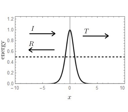
Maple code for quantum scattering from an Eckart potential

One of the more complicated-looking Schrödinger wavefunctions arises from a scattering (i.e., positive energy) problem involving an Eckart potential. These wavefunctions are expressed in terms of Gauss hypergeometric functions and as part of some numerical work I was doing using Maple software I wanted to see how easy or difficult it would be to write a Maple procedure that would compute and plot these objects. It turned out to be not too difficult and I want to record this Maple code in the present note. The following diagram illustrates the basic setup for scattering from an Eckart potential that will be considered here.

The Eckart potential was first introduced in 1930 (Eckart, C, 1930, The penetration of a potential barrier by electrons, Phys Rev 35, Issue 11, pp. 1303-1309) and has the form

$V(x) = \frac{V_0}{\cosh^2\big(\frac{x}{a}\big)}$

where $V_0$ is the height of the potential at the origin and $a$ is its width. We assume that a travelling wave of predetermined amplitude $I$ is moving from left to right towards the origin, corresponding to a free particle of mass $m$ and energy $E$ , where $0 < E < V_0$ . The particle is scattered in the region around the origin where the potential is nonzero, being reflected with probability $R$ and transmitted (by quantum tunnelling, since $E < V_0$ ) with probability $T$ . Usually, the main focus in scattering problems is on the calculation of $R$ (called the reflection coefficient) and $T$ (called the transmission coefficient) for different energy levels.

The time-independent Schrödinger equation for scattering from an Eckart potential of this form can be written as

$-\frac{\hbar^2}{2m} \frac{d^2\psi}{dx^2} + \bigg[\frac{V_0}{\cosh^2\big(\frac{x}{a}\big)} - E\bigg]\psi = 0$

To rescale this for numerical work we can divide through by $-\frac{\hbar^2}{m}$ to get

$\frac{1}{2} \frac{d^2\psi}{dx^2} + [E^{\prime} - V^{\prime}]\psi = 0$

where

$E^{\prime} = \frac{mE}{\hbar^2}$

and

$V^{\prime} = \frac{mV_0}{\hbar^2 \cosh^2\big(\frac{x}{a}\big)}$

To obtain $E^{\prime}$ explicitly, we observe that far away from the origin the potential is zero, so the above equation reduces to

$\frac{d^2\psi}{dx^2} + 2E^{\prime}\psi = 0$

This is a second-order linear ordinary differential equation with a travelling wave solution of the general form

$\psi = Ae^{i\sqrt{2E^{\prime}}x} + Be^{-i\sqrt{2E^{\prime}}x}$

where $k = \sqrt{2E^{\prime}}$ is the wavenumber. We are free to assign any positive value we like to the wavenumber $k$ in scattering problems. This choice of $k$ will then determine $E^{\prime}$ and $E$ . To begin with, we will set $k = 1$ here, which implies $E^{\prime} = \frac{1}{2}$ .

To obtain $V^{\prime}$ explicitly, we note that we are able to assign any value we like to $V_0$ and $a$ so, to begin with, we will choose $V_0 = \frac{\hbar}{m}$ and $a = 1$ to give us the rescaled potential

$V^{\prime} = \frac{1}{\cosh^2(x)}$

which is of unit height and width. This is the setup shown in the diagram above. Therefore the scattering equation we will be implementing to begin with is

$\frac{1}{2} \frac{d^2\psi}{dx^2} + \bigg[\frac{1}{2} - \frac{1}{\cosh^2(x)}\bigg]\psi = 0$

This quantum system can be solved exactly in terms of Gauss hypergeometric functions of the form ${}_2F_1\big([\alpha, \beta], [\gamma], z\big)$ , i.e., with two upper parameters, $\alpha$ and $\beta$ , and one lower parameter, $\gamma$ . (For details, see ter Haar, D, 1975, Problems in quantum mechanics, London: Pion, Chapter 1, Problem 14, Chapter 2, Problem 8, and also Blinder, S, 2011, Scattering by a Symmetrical Eckart Potential, Wolfram Demonstrations Project). Here we will focus on adapting the (rather complicated) exact solution to the case specified above. Given the four parameters $a$ , $V_0$ , $m$ and $k = \frac{\sqrt{2mE}}{\hbar}$ , let

$\lambda = \frac{1}{4}\bigg[\sqrt{1 - \frac{8mV_0a^2}{\hbar^2}} - 1\bigg]$

$a_1 = \frac{\sqrt{\pi}\cdot \Gamma(-ika)}{\Gamma\big(-\lambda - \frac{ika}{2}\big) \cdot \Gamma\big(\lambda + \frac{1}{2} - \frac{ika}{2}\big)}$

$a_2 = \frac{\sqrt{\pi}\cdot \Gamma(-ika)/2}{\Gamma\big(-\lambda + \frac{1}{2} - \frac{ika}{2}\big) \cdot \Gamma\big(\lambda + 1 - \frac{ika}{2}\big)}$

Then the exact solution of the general time-independent Schrödinger equation for this problem is the wavefunction

$\psi = \bigg[\cosh^2\bigg(\frac{x}{a}\bigg)\bigg]^{-2\lambda}\cdot{}_2F_1\bigg(\bigg[-\lambda+\frac{ika}{2}, -\lambda - \frac{ika}{2}\bigg], \bigg[\frac{1}{2}\bigg], -\sinh^2\bigg(\frac{x}{a}\bigg)\bigg)$

$-\frac{a_1}{a_2} \bigg[\cosh\bigg(\frac{x}{a}\bigg)\bigg]^{-2\lambda} \cdot \sinh\bigg(\frac{x}{a}\bigg)\cdot{}_2F_1\bigg(\bigg[-\lambda+\frac{ika}{2}+\frac{1}{2}, -\lambda - \frac{ika}{2}+\frac{1}{2}\bigg], \bigg[\frac{3}{2}\bigg], -\sinh^2\bigg(\frac{x}{a}\bigg)\bigg)$

The exact solution for our particular specifications is then obtained by setting $a = 1$ , $V_0 = 1$ , $m = 1$ and $k = 1$ in this wavefunction. This solution has both real and imaginary parts which are plotted together in the diagram below.

The reflection and transmission coefficients for this scattering problem are given by the formulas

$R = \frac{\cosh^2\bigg(\frac{\pi}{2}\cdot\sqrt{\big|1 - \frac{8mV_0a^2}{\hbar^2}\big|}\bigg)}{\sinh^2(\pi k a)+\cosh^2\bigg(\frac{\pi}{2}\cdot\sqrt{\big|1 - \frac{8mV_0a^2}{\hbar^2}\big|}\bigg)}$

$T = \frac{\sinh^2(\pi k a)}{\sinh^2(\pi k a)+\cosh^2\bigg(\frac{\pi}{2}\cdot\sqrt{\big|1 - \frac{8mV_0a^2}{\hbar^2}\big|}\bigg)}$

Evaluating these with $a = 1$ , $V_0 = 1$ , $m = 1$ , $k = 1$ and $\hbar = 1$ we get a probability of reflection $R = 0.88$ and a probability of transmission $T = 0.12$ .

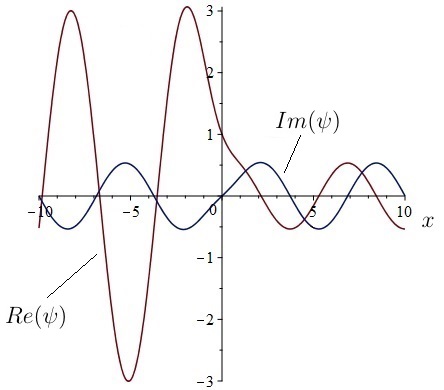
I produced the above wavefunction plot, and calculated the corresponding reflection and transmission probabilities, using the following Maple code:

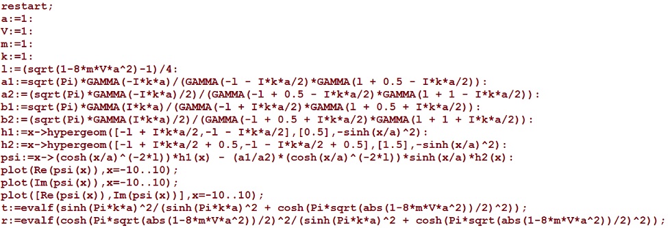
Wavefunction plots and reflection and transmission probabilities for different Eckart scattering parameters can now easily be obtained by simply varying the parameters $a$ , $V$ , $m$ and $k$ in the above code.

2 thoughts on “Maple code for quantum scattering from an Eckart potential”

Boris Sidorenko says:

15th Nov 2024 at 7:18 am

The expression for wave function is a little bit incorrect. In the second addendum a multiplier with cosh should be exponentiation -2*lambda

1. Dr Christian P. H. Salas says:
  
  15th Nov 2024 at 8:14 am
  
  Hi Boris. Thank you for pointing out this typo. I have added the missing exponent to cosh in the second term of the wave function. (Luckily, I did not miss out this exponent when later implementing the wave function in MAPLE).