A mathematics and physics `scrapbook', with notes on miscellaneous things that catch my interest in a range of areas including: mathematical methods; number theory; probability theory; stochastic processes; mathematical economics; econometrics; quantum theory; relativity theory; cosmology; cloud physics; statistical mechanics; nonlinear dynamics; electronic engineering; graph and network theory; mathematics in Latin; computational mathematics using Python and other maths software.
For a lecture on deterministic and stochastic general epidemic models, I ran a Python simulation illustrating a threshold phenomenon which determines how an epidemic evolves. I want to record the results of this here.
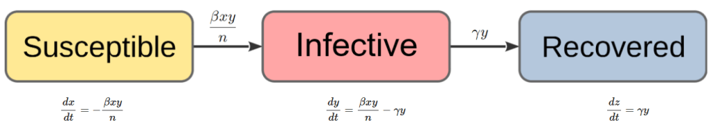
In a general epidemic model, we assume a closed community of individuals and classify those individuals into three groups, those who are susceptible to disease, those who are infective, and those who are removed (i.e., who have had the disease and are no longer infective). The numbers of each type at time are denoted by , and respectively. Note that since , the time evolution of is automatically determined by the evolution of and . At any given time , only two types of transition are possible. The first type of transition is SUSCEPTIBLE INFECTIVE in which an infective meets a susceptible and the disease is passed on, causing the number of susceptibles to decrease by one and the number of infectives to increase by one. The second type of transition is INFECTIVE REMOVED in which an infective recovers from the disease, so the total number of infectives decreases by one and the total number removed increases by one.
Assuming that each member of the community comes into contact with the remaining others according to a Poisson process with rate , that there is homogenous mixing so that the probability of one member meeting any other particular member is , and that a susceptible who becomes infected with the disease only remains infective for a time drawn from an exponential distribution with rate , then the general epidemic as a stochastic process can be characterised by the following two probability statements corresponding to the two types of transitions outlined above:
The first probability statement says that infectives meet susceptibles according to a Poisson process with rate , while the second probability statement says that infectives recover and become removed according to a Poisson process with rate , where and denote realised numbers of susceptibles and infectives at time respectively.
To obtain a deterministic approximation of the above stochastic general epidemic model, we set up ordinary differential equations for the time evolution of , and based on the probability statements (1) and (2). From (1), we see that susceptibles decrease at the rate and infectives correspondingly increase at the same rate, while from (2) we see that infectives also decrease at the rate and the removed correspondingly increase at the same rate. We thus get the following system of three coupled ordinary differential equations for the deterministic general epidemic model:
These cannot generally be solved to get explicit expressions for , and as functions of time, but can be solved numerically to get time paths for these variables, as shown below using Python. It is also straightforward to obtain a differential equation for in terms of by dividing (4) by (3) to get
where
is a key parameter known as the epidemic parameter. The differential equation (6) can easily be solved given initial conditions , , , to get an equation for in terms of :
This equation describes the evolution of the epidemic in a `timeless’ way in the -plane and predicts that the epidemic parameter plays a crucial role. It acts as a threshold parameter in the following sense: if , the number of infectives never rises above the initial number and in fact declines steadily from there until it reaches at which point the epidemic ends (since there are no more infectives to pass on the disease), whereas if , the number of infectives can rise significantly above until it reaches a maximum value before beginning to decline from there until the epidemic ends again when . Public health measures therefore aim to reduce the number of susceptibles (e.g., by immunisation) and to increase the value of the epidemic parameter by increasing the removal rate and decreasing the contact rate (e.g., by encouraging self-isolation) to try to achieve a scenario in which .
To supplement these results, I wanted to use Python to get time paths for , and as direct numerical solutions to the coupled differential equations (3), (4) and (5), ideally also demonstrating the threshold phenomenon with these time paths. The following diagram summarises the deterministic general epidemic model to be implemented in Python:
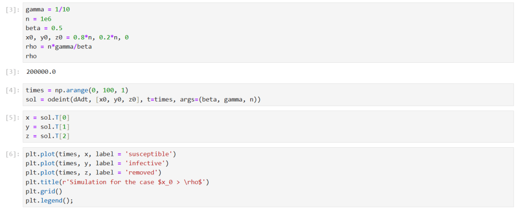
I used the odeint() function from the scipy.integrate library to solve the differential equation system numerically. This requires the definition of a Python function which takes as inputs , , , and , and returns the vector derivative .
First, I ran a simulation for the case . I solved the model equations for
Note that the corresponding epidemic parameter is .
The results show the classic epidemic pattern for , with the number of infectives rising significantly above before declining to . Note that almost all the susceptibles ended up being infected in this scenario.
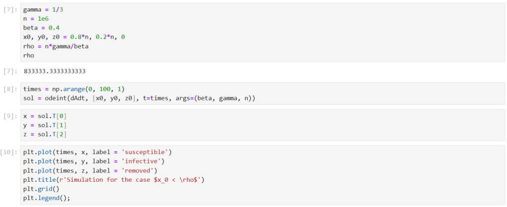
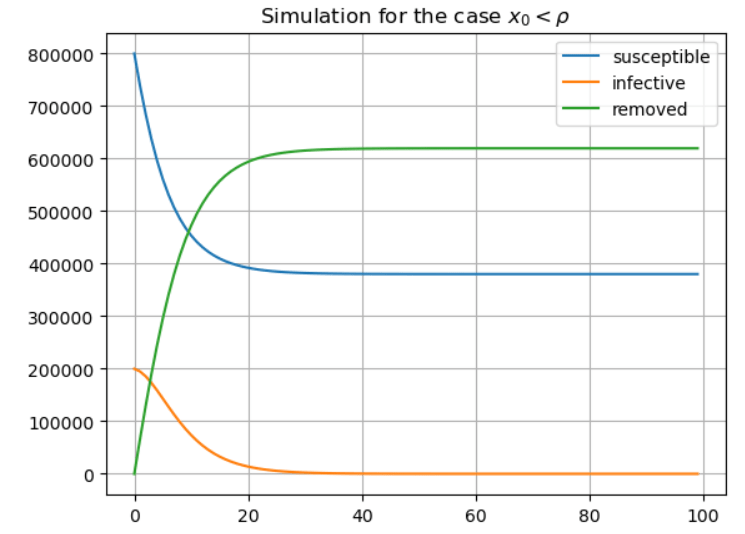
Next, I ran a simulation for the case . Suppose that public health measures have managed to increase the value of the epidemic parameter by increasing the removal rate and reducing the contact rate . I solved the model equations for
Note that the corresponding epidemic parameter is now .
The results now show the typical results for , with the number of infectives never rising above the initial , and declining steadily to . Note that almost half of the initial number of susceptibles remained unaffected by the disease in this scenario.
The M/M/1 queue is the simplest Markov queueing model, and yet it is already sufficiently complicated to make it impractical in an introductory queueing theory lecture to derive time-dependent probability distributions for random variables of interest such as queue size and queueing time. A simpler approach is to assume the queue eventually reaches a steady state, and then use the forward Kolmogorov equations under this assumption to obtain equilibrium expected values of relevant random variables.
For the purposes of a lecture on this topic, I wanted to run some simulations of M/M/1 queues using Python to get a feel for how quickly or otherwise they actually reach their equilibrium. I was expecting equilibration after a few tens or hundreds of customers had passed through the queue. To my surprise, however, I ended up doing simulations involving a million customers and it typically took a few hundred thousand before the queue converged to theoretically predicted equilibrium values of things like mean queue size and mean queueing time. I want to record the relevant calculations and Python simulations here.
In M/M/1 queues, arrivals of customers occur according to a Poisson process with rate , there is a single server, and departures occur according to a Poisson process with rate (so, the service time for each customer is exponentially distributed, also with rate ). Suppose the queue contains customers at time where is a small time increment. Given the axioms of a Poisson process, there are only three possibilities for the number of customers at time :
There could have been customers at time and one departed, or there could have been customers at time and one arrived, or there could have been customers at time and there were no departures or arrivals. By the axioms of a Poisson process, these three possibilities have probabilities
for the cases . In the case , we have
since a departure is impossible when there are no customers in the queue.
The M/M/1 queue is a continuous-time Markov process for which Chapman-Kolmogorov equations can be obtained by applying the Theorem of Total Probability. The Chapman-Kolmogorov equations say that
where is the number of customers at time 0 and the summation is over all relevant states in the state space. The only relevant states here are , , and as outlined above, so the Chapman-Kolmogorov equations for the current situation are
Rearranging, we get
Letting , we get the Kolmogorov forward equations for the M/M/1 queue:
for the cases , and
for the case .
These equations can be solved to get a time-dependent probability distribution for the queue size, but the procedure is far from straightforward and the time-dependent probability distribution itself is very complicated. What can be done far more easily is to assume that the process reaches a steady state after many customers have arrived and departed, and then calculate the expected values of random variables of interest such as the expected queue size and the expected queueing time. This is what we will do here, before confirming the calculations using Python simulations.
When the process has reached a steady state, the probabilities are no longer changing over time, so we have . Setting the left-hand sides of the Kolmogorov forward equations equal to zero and solving the equations recursively for and then , we get
for , where is called the traffic intensity. For the equilibrium distribution to exist, these probabilities must sum to 1, which requires . In this case, we have
so,
Substituting this into the equation for above we get
which is the probability mass function of a geometric distribution starting at 0 with parameter . The mean queue size in the steady state of this process is the mean of this distribution, which is
It can also be shown fairly straightforwardly that the mean queueing time for the M/M/1 queue in equilibrium is the mean of an exponential distribution with parameter , so the mean queueing time is
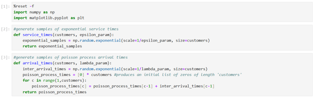
To simulate this M/M/1 queue in Python, we begin by defining Python functions for the exponential service times and Poisson arrivals:
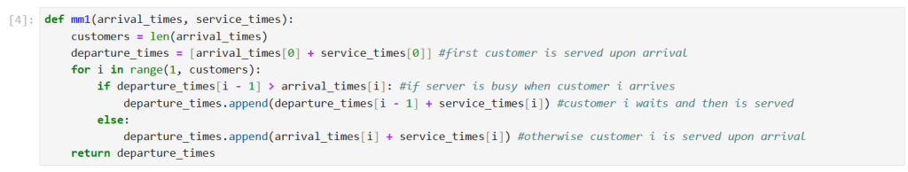
Next, we compute departure times for customers in an M/M/1 queue given the arrival times and service times generated by the previous functions. Each customer is either served upon arrival if the server is free, or has to wait for the previous customer to depart before being served.
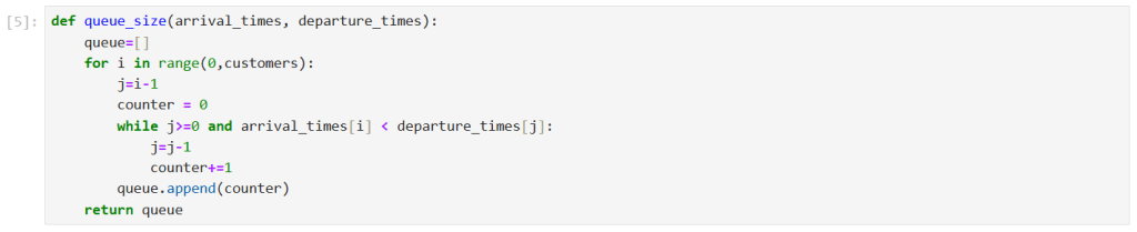
We can also compute queue sizes, given the arrival times and departure times of customers. To clarify the algorithm, suppose we want to know the queue size when customer 5 arrives. We set counter = 0 to initialise it and we set j = 4 to look at customer 4’s departure time. If the arrival time of customer 5 is before the departure time of customer 4, then we know there was at least one person in the queue so we set counter = 1 and change j = 3 to look at customer 3’s departure time. We continue with this process until the arrival time of customer 5 is after the departure time of a previous customer, or until we reach j = 0 at which point we will have counter = 4 if the arrival time of customer 5 is before the departure time of customer 0. We will then set j = -1 and the counting process will stop.
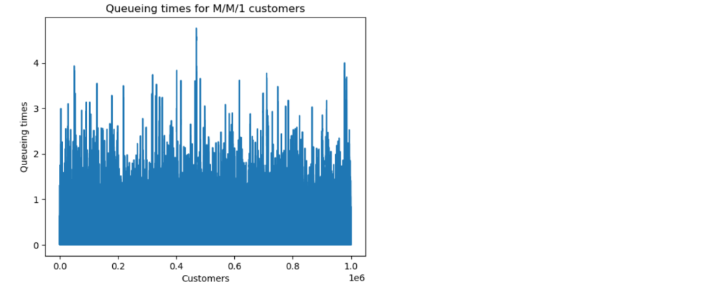
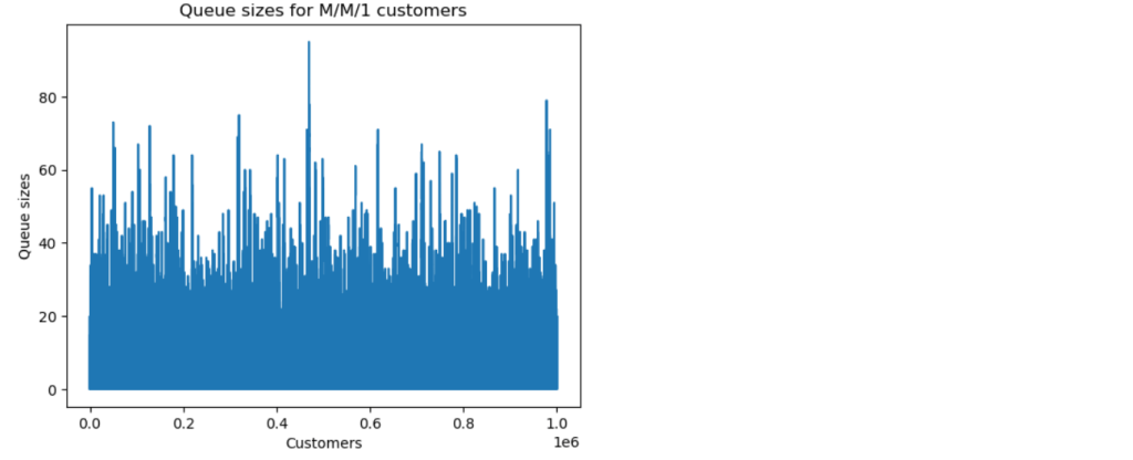
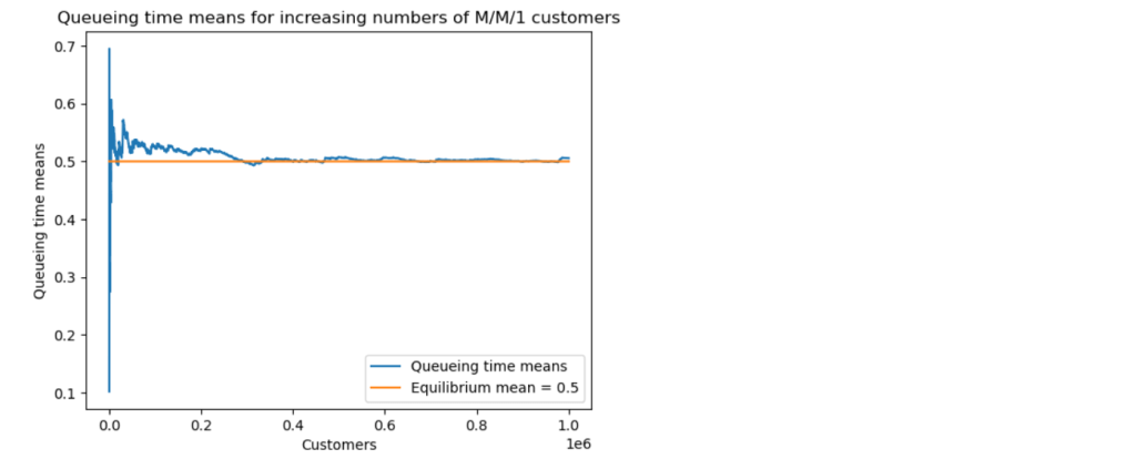
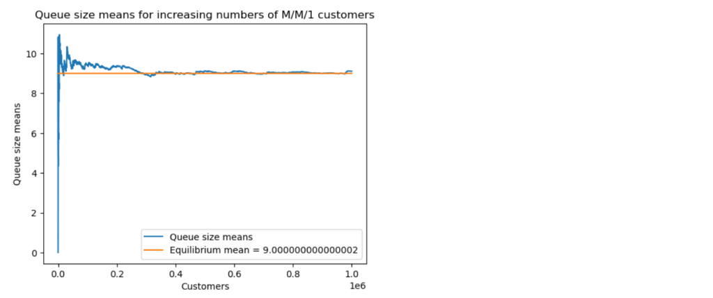
We can now run a simulation. The results below are for a simulation with one million customers, and parameter values and . The predicted equilibrium mean queueing time is time units, and the predicted equilibrium mean queue size is .
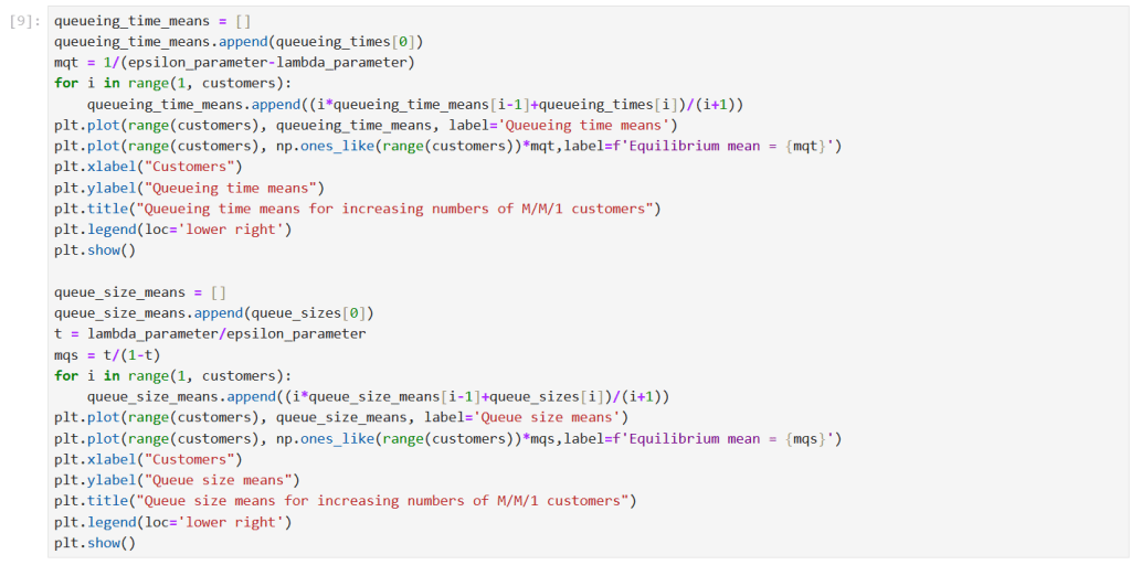
We now explore how long it takes for the M/M/1 queue to settle down to its steady state. We look at the convergence of both the queueing time means and the queue size means to their theoretical equilibrium values.
The simulation with one million customers eventually settled down to the predicted theoretical values for mean queue size and mean queueing time, but this took a surprisingly long time, around 400 thousand customers.
During a lecture on the solution of standard ODEs, a student asked why we use as the solution of the integral in the exponent of an integrating factor rather than the formally correct antiderivative . In particular, the student was concerned about the omission of the modulus symbol around the . The explanation is not an unsubtle one and is often overlooked or treated lightly when this approach is used, so I thought I would record the discussion here.
The first-order ODE under discussion was of the simple form
This can easily be solved using the integrating factor method, with integrating factor
We multiply BOTH sides of the original ODE by this integrating factor to obtain
and then observe that the left-hand side can be written as the derivative of a product:
This is now easy to integrate, and upon integrating both sides with respect to we obtain
which gives the required explicit general solution for :
The question that arose was why we did not use for the integral in (2) above. Is this not the correct antiderivative solution for ?
It is true that when one is finding the general antiderivative of one must give the answer as . However, it is NOT necessary to do this when the integral of appears as the exponent of the integrating factor in a problem like (1). It is also not necessary to include an arbitrary constant in the integral in the exponent of the integrating factor, for the same reason.
This is because, as exemplified above, the integrating factor is something that one multiplies BOTH sides of the differential equation by to enable the left-hand side to be expressed as the derivative of a product. As we saw above, it is then easy to obtain a solution by integrating both sides. Since the integrating factor multiplies both sides of the differential equation, it would make no difference to the final solution if we were to multiply the integrating factor by a constant. Any constant which multiplies the integrating factor would simply cancel out when using the integrating factor method to solve the differential equation.
If we used as the integrating factor in (2), we would obtain the same solution to the differential equation as in (6), irrespective of whether or , because when we have
This is just a constant times the integrating factor obtained in (2), so as described above the constant will cancel out and it will be AS IF we had used the integrating factor in (2) in the first place.
That’s why we just ignore the modulus symbol (and the arbitrary constant) when using the integrating factor method in cases like (1). We don’t need to think of the integral in the exponent of the integrating factor in the same way as we would think of the general antiderivative, because this doesn’t affect the final solution of the differential equation.
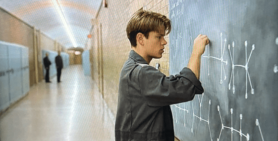
In the cult classic movie Good Will Hunting (Miramax, 1997), a maths-genius janitor played by a young Matt Damon secretly solves challenge problems in graph theory written on a blackboard by an MIT maths professor for his students.
One of these problems, which Will can be seen solving in the above screenshot from the movie, is the following:
Draw all the homeomorphically irreducible trees with n=10.
Homeomorphically irreducible trees are those which do not contain any vertices of degree 2 and which are non-isomorphic. There are ten such 10-node trees, as follows:
There are many articles and videos online which discuss how these ten trees can be deduced in various ways. However, two questions which have always bothered me since I first saw the movie do not seem to have been discussed anywhere. While preparing an introductory lecture on trees in graph theory, I decided to try to answer these questions once and for all and am recording the results in the present post. (I also presented these results in my lecture!)
By Cayley’s famous formula for the number of labelled trees with vertices, there are 100 million labelled 10-node trees. I always wondered how many of these 100 million labelled 10-node trees are irreducible, and how many of the irreducible labelled trees belong to each of the ten homeomorphically irreducible types in the Good Will Hunting problem? Below, I first use combinatorial arguments to calculate the number of irreducible labelled 10-node trees and then confirm this figure using Python. I also use Python to classify the irreducible labelled trees into the ten Good Will Hunting isomorphism classes.
Combinatorial calculations
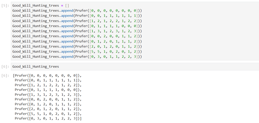
To calculate the total number of irreducible labelled 10-node trees, we begin by observing that the Prüfer sequences of these trees will all be 8 digits long and such that no number occurs with a frequency of 1 (the degree of a vertex in a tree is one more than the frequency of occurrence of the vertex label in the tree’s Prüfer sequence, so the Prüfer sequences of trees which do not contain vertices of degree 2 cannot contain vertex labels with a frequency of 1). To illustrate this, I randomly assigned labels to the ten non-isomorphic trees from the Good Will Hunting problem above and calculated their Prüfer sequences as follows:
As expected, all the vertex labels in the Prüfer sequences above appear with frequencies of at least 2. Therefore, the combinatorial problem we need to solve is the following:
How many ways are there to form a sequence of 8 numbers chosen from the ten numbers 0, 1, 2, 3, 4, 5, 6, 7, 8, 9, in such a way that each number that appears in the sequence appears at least twice?
We will need to use a standard result from combinatorics which says that if there are objects, with of type 1, of type 2, . . . , and of type , where , then the number of arrangements of these objects, denoted , is
To apply this result, we need to identify all the possible patterns of 8-digit arrangements satisfying the above conditions, then apply the formula to each possible pattern to find out how many ways there are to arrange the 8 digits in that pattern. Adding up all the possible ways of arranging the 8 digits in each pattern will then give the total number of irreducible labelled 10-node trees. There are actually only seven cases that need to be considered. Using letters to stand for numbers, only the following seven patterns are possible:
Case 1:
Here, only a single number appears in the Prüfer sequence. There are 10 options for choosing which number occurs 8 times in this sequence, so there are 10 ways to arrange a Prüfer sequence in which one number occurs 8 times.
Case 2:
Here, only two numbers appear in the Prüfer sequence, one of them 6 times and the other 2 times. There are 10 options for choosing which number occurs 6 times and then 9 options for choosing which number occurs 2 times. Using formula (1) above, there are ways to arrange 6 of one number and 2 of the other. Thus, there are ways to arrange a Prüfer sequence in which one number occurs 6 times and another occurs twice.
Case 3:
Here, only two numbers appear in the Prüfer sequence, one of them 5 times and the other 3 times. There are 10 options for choosing which number occurs 5 times and then 9 options for choosing which number occurs 3 times. Using formula (1) above, there are ways to arrange 5 of one number and 3 of the other. Thus, there are ways to arrange a Prüfer sequence in which one number occurs 5 times and another occurs 3 times.
Case 4:
Here, only two numbers appear in the Prüfer sequence, each of them 4 times. There are 10 options for choosing a first number which occurs 4 times and then 9 options for choosing a second number which occurs 4 times. When considering the possible arrangements, we note that the numbers can be interchanged without affecting each given arrangement because they occur with the same frequency, so there are two equivalent versions of each arrangement. Thus, using formula (1) above, there are ways to arrange 4 of one number and 4 of the other. Thus, there are ways to arrange a Prüfer sequence in which one number occurs 4 times and another occurs 4 times.
Case 5:
Here, three different numbers appear in the Prüfer sequence, one of them 4 times and the other two twice. There are 10 options for choosing a first number which occurs 4 times, then 9 options for choosing a second number which occurs 2 times, then 8 options for choosing a third number which occurs 2 times. When considering the possible arrangements, we note that the two numbers which occur twice can be interchanged without affecting each given arrangement because they occur with the same frequency, so there are two equivalent versions of each arrangement. Thus, using formula (1) above, there are ways to arrange 4 of one number and 2 of each of the other two numbers. Thus, there are ways to arrange a Prüfer sequence in which one number occurs 4 times and two other numbers occur 2 times each.
Case 6:
Here, three different numbers appear in the Prüfer sequence, one of them 2 times and the other two 3 times. There are 10 options for choosing a first number which occurs 2 times, then 9 options for choosing a second number which occurs 3 times, then 8 options for choosing a third number which occurs 3 times. When considering the possible arrangements, we note that the two numbers which occur 3 times can be interchanged without affecting each given arrangement because they occur with the same frequency, so there are two equivalent versions of each arrangement. Thus, using formula (1) above, there are ways to arrange 2 of one number and 3 of each of the other two numbers. Thus, there are ways to arrange a Prüfer sequence in which one number occurs 2 times and two other numbers occur 3 times each.
Case 7:
Finally, four different numbers appear in this case, each of them 2 times. There are 10 options for choosing a first number which occurs 2 times, then 9 options for choosing a second, then 8 options for choosing a third, then 7 options for choosing the fourth. When considering the possible arrangements, we note that the four numbers which occur 2 times can be interchanged without affecting each given arrangement because they occur with the same frequency, so there are equivalent versions of each arrangement. Thus, using formula (1) above, there are ways to arrange 2 each of four numbers. Thus, there are ways to arrange a Prüfer sequence in which four different numbers occur 2 times each.
Adding up the totals for the seven cases above, we find
Thus, according to the combinatorial calculation approach above, there are 892720 irreducible labelled 10-node trees. This will now be confirmed computationally using Python, and the 892720 trees will also be classified into the ten Good Will Hunting isomorphism types.
Python calculations
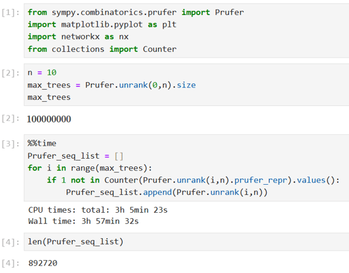
To confirm the number of irreducible labelled 10-node trees, I wrote the following Python code to pick from the 100 million labelled 10-node trees those whose Prüfer sequences do not contain vertex labels with a frequency of 1. As can be seen from the output, this took nearly 4 hours (on a laptop with 16.0GB of RAM) and confirmed the number 892720 obtained via the combinatorial calculations above.
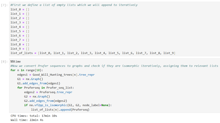
I then wrote the following Python code to classify the 892720 irreducible trees into the ten Good Will Hunting isomorphism types. This code uses the Prüfer sequences I calculated for the randomly labelled ten isomorphism types above as templates against which each of the 892720 trees can be checked. Each tree is then classified into one of the ten types depending on which of the ten Prüfer sequences it is isomorphic to.
As can be seen from the output here, this classification process took 22 minutes. The results showing the classification of the 892720 trees into the ten Good Will Hunting isomorphism types are shown below, together with a check that the ten totals do indeed account for all the 892720 irreducible trees.
For a lecture on digraphs and network flows, I prepared the following capacitated directed network problem in order to explore its solution both manually via a maximum-flow/minimum-cut algorithm and computationally using the NetworkX library in Python:
The number on each arc represents the flow capacity of that arc and the vertices and are the source and the sink for the flow respectively (all arcs containing are directed away from and all arcs containing are directed towards ).
The max-flow/min-cut algorithm involves a labelling procedure which, starting from an initial flow (e.g., a zero flow) enables augmentation of flows along some arcs as well as reduction of flows along others. The idea is to increase the flow from to as much as possible subject to the capacity constraints on the arcs by using the algorithm to keep finding flow-augmenting routes through the network. The process terminates when all flow-augmenting routes have been found and a maximum flowvalue for the network thus becomes known. The algorithm will also result in some of the arcs in the network becoming saturated, i.e., filled to capacity, and a set of arcs containing some of these saturated arcs will constitute a minimum cut for the network. Such a minimum cut is a set of arcs with the smallest possible sum of capacities such that removal of all the arcs in the set divides the network into two disjoint parts and , the part containing the source and the part containing the sink . A theorem known as the max-flow min-cut theorem states that the maximum flow value must equal the capacity value of the minimum cut for a basic network such as the one in the diagram above. Finding a minimum cut using the saturated arcs at the end of the algorithm thus provides a useful way to check that the final flow is indeed a maximal one.
Below, I will solve the above problem both manually and using the NetworkX library in Python. For the manual solution, I will use a labelling procedure to record movement from one vertex to the next vertex with the notation , where is the size of flow that is possible along the arc subject to the capacity of the arc and also subject to the possible flow at the previous step. Where there is a choice of arc when moving from one vertex to the next, we choose alphabetically. When moving backwards along an arc, this is indicated with a minus sign so that, for example, indicates that we moved from to along an arc that was actually directed from to .
The manual solution is a little burdensome mainly because it requires making repeated copies of the network showing the adjustments at each step of the algorithm. Below I will render these copies by hand. At each step, each arc is labelled with two numbers separated by a comma, the first number being the flow along the arc and the second being the capacity of the arc. I will highlight that an arc is saturated by thickening the line representing the arc. We assume a zero initial flow, represented as follows in a manual copy of the above network:
Starting from vertex , we choose alphabetically the arc . The labels are: . The path is . The flow increase is . The saturated arc is . Making these amendments, the network looks as follows after this first run:
For the next run, we begin again with arc . The labels are: . The path is . The flow increase is . The saturated arc is . The network looks as follows after this second run:
We begin again with arc . The labels are: . The path is . The flow increase is . The saturated arc is . The network looks as follows after this third run:
We begin again with arc . The labels are: . The path is . The flow increase is . The saturated arc is . The network looks as follows after this fourth run:
We begin again with arc . The labels are: . The path is . The flow increase is . The saturated arc is . The network looks as follows after this fifth run:
Proceeding alphabetically, we now begin with arc . The labels are: . The path is . The flow increase is . The saturated arcs are and . The network looks as follows after this sixth run:
We begin again with arc . The labels are: . The path is . The flow increase is . The saturated arc is . The network looks as follows after this seventh run:
We begin again with arc . The labels are: . The path is . The flow increase is . The saturated arcs are and . The network looks as follows after this eighth run:
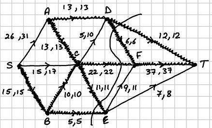
Proceeding alphabetically, we now begin with arc . The labels are: . The path is . The flow increase is . The saturated arc is . The network looks as follows after this ninth run:
We begin again with arc . The labels are: . The path is . The flow increase is . The saturated arc is . The network looks as follows after this tenth run:
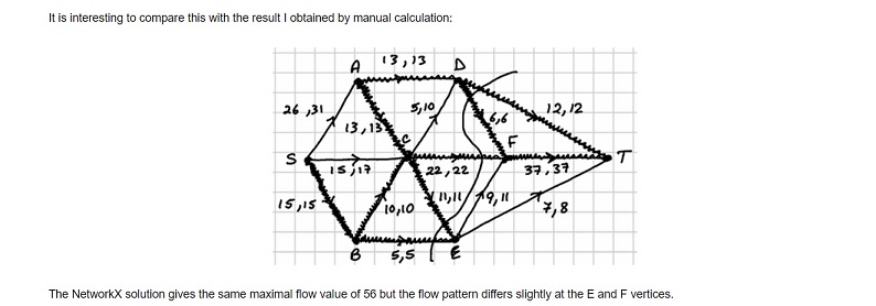
The algorithm is now complete. The diagram below shows the maximum flow and a minimum cut for this network:
The maximum flow has the value . The minimum cut is the set of arcs which has capacity .
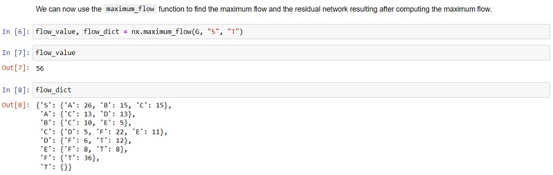
Having solved the problem manually, it is interesting to now compare this solution with a computational solution produced using the library NetworkX in Python. I did the coding for this problem in a Jupyter Notebook as follows:
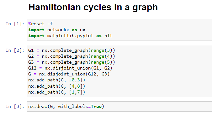
For the purposes of a lecture in graph theory, I created the following example of a Hamiltonian graph consisting of the complete graphs , and joined pairwise by an edge:
The Python library NetworkX can be used to perform many of the calculations that arise in graph theory and networks and I used it in this case to list and count all the Hamiltonian cycles in the above graph. In the present post, I want to quickly record the Python code I used for this (in a Jupyter Notebook):
Consider a so-called canonical ensemble consisting of a system , a heat bath , and the total closed system containing and , with corresponding energies , and respectively so that
with fixed. For example, could represent a single 1-D lattice of spins in the Ising Model, could consist of a heat bath with which is in thermal contact, and would be the closed system containing and .
With regard to the 1-D lattice of spins, different spin configurations will have different energies and for a given energy there will be a multiplicity of spin configurations with that same energy (i.e., if is the macrostate, there will be different microstates yielding that same macrostate). Similarly, if the energy is the macrostate of the heat bath, there will be different microstates yielding that same macrostate. Since is fixed, we see that the total number of microstates for the combined system, , is a function of :
Suppose we pick one particular spin configuration of the 1-D lattice of spins with associated energy . Then and because we have picked a particular microstate for system . We will now obtain from this setup the probability of the combined system being in this state. The total number of microstates for the combined system is now
The entropy of the combined system using Boltzmann’s entropy equation is
where is the Boltzmann constant.
To obtain an expression for the temperature of the heat bath, we can use the first law of thermodynamics which in the absence of any work done by the system reduces to
where is the internal energy of the system and is energy added via heat. Using the differential form of the definition of entropy in thermodynamics, namely
we get from (5) that
Using (7) with (4) we then have
Integrating gives
where is an integration constant. Therefore, we have
This calculation is for one particular energy level, , of the 1-D lattice of spins. Summing over all possible energy levels, the total number of microstates of the combined system is
The probability of the combined system being in state is then obtained by dividing (10) by (11):
This is the Boltzmann probability distribution, with
being the partition function. Note that all terms involving the heat bath end up dropping out. The only relevance of the heat bath is to define the temperature of the system. Everything else about it is irrelevant.
The 1-D lattice of spins does not have constant energy when it is in contact with a heat bath. The energy of the system fluctuates with probabilities governed by the Boltzmann distribution. We can obtain a formula for the average entropy of the 1-D lattice of spins in the canonical ensemble, called the Gibbs-Shannon entropy, in terms of Boltzmann probabilities. Imagine taking many measurements of the energy of the 1-D lattice of spins. Interpreting as a relative frequency, the multiplicity of microstates giving energy is
The entropy of the configuration giving rise to energy is then
The Gibbs-Shannon average entropy is obtained from (15) as
Note that (16) simplifies to Boltzmann’s formula for the entropy when all the probabilities are equal, say
for all , since then we have
Finally, we can obtain the Helmholtz free energy by taking logarithms of the Boltzmann probability in (12) to get
Substituting this into the Gibbs-Shannon entropy formula in (16) we get
which can be rewritten as
The quantity is the average value of the Helmholtz free energy, , which is a function of state, i.e., it is a function only of macroscopic thermodynamic variables. The equation
linking the free energy to the partition function is therefore of vital importance since it relates the large-scale properties of the system to its microscopic energy states. The partition function acts like a bridge between these two regimes.
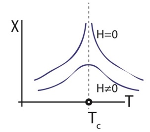
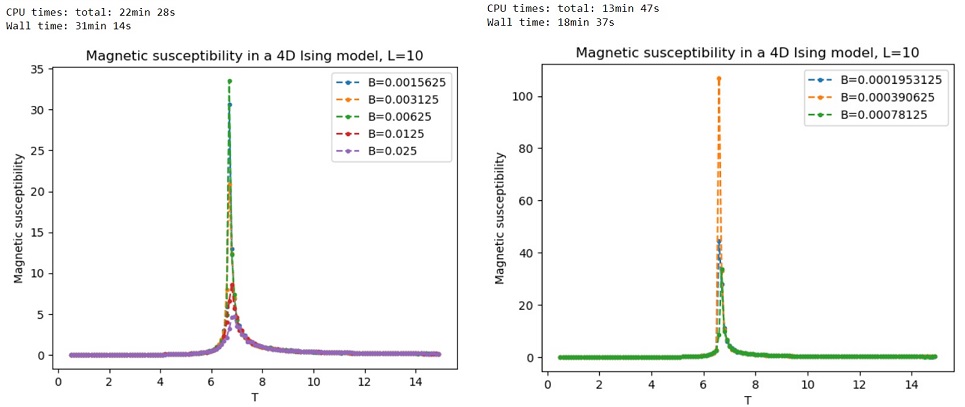
For the purposes of a lecture on simulating the Ising model of ferromagnetism using the Metropolis-Hastings algorithm, I explored the behaviour of magnetic susceptibility on a four-dimensional hypercube lattice. In particular, I wanted to test a well-known prediction of theoretical physics that a zero-field singularity should appear at a certain critical temperature. The idea is that there is an essential singularity in the mathematics at zero external magnetic field which disappears with a non-zero magnetic field. See the discussion on physics Stack Exchange about this. I was interested to see if a computer simulation of magnetic susceptibility in an Ising model on a four-dimensional hypercube lattice would produce similar results as the second diagram in this Stack Exchange query, which I reproduce here:
The results do suggest that, in the nearest-neighbour ferromagnetic Ising model on a 4-D hypercube lattice, there is a cusp-like singularity in magnetic susceptibility at a critical temperature around T = 7. This singularity becomes more and more apparent in the plots as the external magnetic field strength is reduced to zero but tends to disappear as the field strength increases. I want to record this experiment and the results in the present post.
I considered a 4-D ferromagnetic Ising model on a hypercubic lattice, with . I assumed periodic boundary conditions and the presence of an external magnetic field with parameter . The nearest-neighbour Hamiltonian for a particular configuration of the spins on the four-dimensional hypercube is
where is the spin at site on the lattice, is the nearest-neighbour interaction energy and is the external magnetic field parameter. The partition function assuming thermal equilibrium at a temperature is
where is Boltzmann’s constant and is the Hamiltonian for the -th spin configuration . For the computer simulations I used units in which and .
I used Monte Carlo simulations in the form of the well-known single-flip Metropolis-Hastings algorithm to produce plots of the magnetic susceptibility, , as a function of the temperature in the range to , for a lattice of size with , and . With units in which and , the magnetic susceptibility is calculated as
where
is the total magnetisation given a particular spin configuration on the 4-D lattice.
I initially chose a range of -values rising from to in multiples of two. I obtained the following results for , and , starting with a completely ordered configuration in which all the spins in the lattice were in the state:
The results show a clear peak in magnetic susceptibility becoming more pronounced as is reduced towards zero, with the critical temperature being around . Notice also a rapid increase in the CPU time with , the CPU time being around one minute for , twelve minutes for , and over two hours for . The plot did not change much between and so I used for the remaining simulations.
To confirm the zero-field singularity at the critical temperature , I reduced even further. I obtained the following plots for -values going down to .
It is clear that the peak becomes arbitrarily large as at a critical temperature of around , indicating that there is indeed a singularity there.
Then it is straightforward to show that the Fourier transform of the scaled function is
and the Fourier transform of the -translated function is
What is a little less straightforward is to deduce from these what the Fourier transform must be of a function that has been both scaled and translated in the form
In fact, the Fourier transform of this particular type of scaled and translated function is a simple combination of the two individual adjustments as if they had occurred independently of each other:
We should be able to deduce this by performing the calculations for the scaling and translation sequentially, and we should get the same answer irrespective of the order in which the transformations are performed. However, there are subtleties involved and these are what I am interested in recording in the present note.
Consider performing the scaling first and then the translation. Let so that . Then the combined transformation in (2) is obtained as which has Fourier transform
This agrees with (3). However, when going the other way and performing the translation first before the scaling, it is necessary to remember that the translation in (2) is by an amount . Therefore, in this case, we have to let so that . Then the combined transformation in (2) is obtained as which has Fourier transform
This again agrees with (3), but this way round we see that there has had to be a process of cancellation of the parameter in the complex exponential term. This complication is avoided by performing the scaling first before the translation, making this particular ordering of the transformations a little easier to work with in the case of the combined transformation in (2).
The Ornstein-Uhlenbeck process is widely used in the stochastic modelling of mean-reverting processes. In the present note, I want to record a derivation I produced for a lecture of the pdf and moments of an Ornstein-Uhlenbeck process exhibiting mean-reversion to zero with a stochastic differential equation (SDE) of the form
where and are constants and is a standard Wiener process. I used the Euler–Maruyama method with a time step of in Python to generate and plot a sample path of this process from up to , setting the initial position as and the values and . The following picture shows this sample path:
The mean-reversion to zero is clear from the plot and arises due to the parameter in the drift term of the SDE, which tends to pull the process back down when goes above zero and back up when goes below zero.
The Fokker-Planck equation of the SDE in (1) is easily obtained as
and this can be used to derive a stationary pdf for the Ornstein-Uhlenbeck process corresponding to a long-term equilibrium situation in which the pdf is not time-varying, so . From (2) we then get
Equation (3) tells us that the sum of the two terms in the square brackets must be equal to a constant. Setting this constant equal to zero gives us
and so
from which we deduce the form of the stationary pdf to be
We can find an expression for from the normalisation condition
Making the change of variable we can rewrite (4) as
from which we get
where
The moments of the Ornstein-Uhlenbeck process are obtained as
Making the change of variable , we have and . Using these substitutions together with the expression for in (5) above we get
where
From (8), we see that the first two moments of the Ornstein-Uhlenbeck process are
and
These can be computed directly in Python using code such as the following (quad is from the scipy.integrate library):
This is useful to know for more complicated stochastic processes where the integrals , and might be difficult to evaluate manually, but in the case of the Ornstein-Uhlenbeck process these three integrals have simple exact values. For in (6), we use the well-known trick of solving the double integral
Changing to polar coordinates and , with limits to for and to for , and the Cartesian area element becoming the polar coordinates area element , the double integral becomes
Since (12) is the square of , we conclude . It is easily shown that , and we can calculate by integrating by parts:
Thus,
We can therefore write the first two moments of the Ornstein-Uhlenbeck process with the SDE in (1) above in exact form as
and
To check these calculations, I used Python to compute sample paths of the Ornstein-Uhlenbeck process with the same specifications as the plot above, and plotted the mean and mean squared distance as functions of time together with the corresponding exact values. The plots below show that for sufficiently long times the numerical calculations do indeed fluctuate around the values predicted on the basis of the stationary pdf derived above:
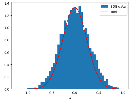
I also calculated the histogram of the probability density of the random variable evaluated at using the simulated sample paths, and plotted it together with the stationary pdf, , derived above from the Fokker-Planck equation. The plot below shows good agreement between the two:


 , there is a single server, and departures occur according to a Poisson process with rate
  (so, the service time for each customer is exponentially distributed, also with rate
  where
where  is a small time increment. Given the axioms of a Poisson process, there are only three possibilities for the number of customers at time
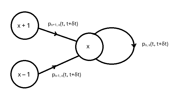
 customers at time
  customers at time


 . In the case
  , we have


 is the number of customers at time 0 and the summation is over all relevant states
  in the state space. The only relevant states


 , we get the Kolmogorov forward equations for the M/M/1 queue:

 are no longer changing over time, so we have
  . Setting the left-hand sides of the Kolmogorov forward equations equal to zero and solving the equations recursively for
  , we get
 , where
  is called the traffic intensity. For the equilibrium distribution to exist, these probabilities must sum to 1, which requires
  . In this case, we have

 above we get

 , so the mean queueing time is
 and
and  . The predicted equilibrium mean queueing time is
  time units, and the predicted equilibrium mean queue size is
  .
. 
 as the solution of the integral
  in the exponent of an integrating factor rather than the formally correct antiderivative
  . In particular, the student was concerned about the omission of the modulus symbol around the


 for the integral in (2) above. Is this not the correct antiderivative solution for
  ?
?  one must give the answer as
  as the integrating factor in (2), we would obtain the same solution to the differential equation as in (6), irrespective of whether
  or
or  , because when

 for the number of labelled trees with
  vertices, there are 100 million labelled 10-node trees. I always wondered how many of these 100 million labelled 10-node trees are irreducible, and how many of the irreducible labelled trees belong to each of the ten homeomorphically irreducible types in the Good Will Hunting problem? Below, I first use combinatorial arguments to calculate the number of irreducible labelled 10-node trees and then confirm this figure using Python. I also use Python to classify the irreducible labelled trees into the ten Good Will Hunting isomorphism classes.
 of type 1,
  of type 2, . . . , and
  of type
  , where
  , then the number of arrangements of these objects, denoted
  , is
, is


 ways to arrange 6 of one number and 2 of the other. Thus, there are
  ways to arrange a Prüfer sequence in which one number occurs 6 times and another occurs twice.
 ways to arrange 5 of one number and 3 of the other. Thus, there are
  ways to arrange a Prüfer sequence in which one number occurs 5 times and another occurs 3 times.
 ways to arrange 4 of one number and 4 of the other. Thus, there are
  ways to arrange a Prüfer sequence in which one number occurs 4 times and another occurs 4 times.
 ways to arrange 4 of one number and 2 of each of the other two numbers. Thus, there are
  ways to arrange a Prüfer sequence in which one number occurs 4 times and two other numbers occur 2 times each.
 ways to arrange 2 of one number and 3 of each of the other two numbers. Thus, there are
  ways to arrange a Prüfer sequence in which one number occurs 2 times and two other numbers occur 3 times each.
 equivalent versions of each arrangement. Thus, using formula (1) above, there are
  ways to arrange 2 each of four numbers. Thus, there are
  ways to arrange a Prüfer sequence in which four different numbers occur 2 times each.


 and
and  are the source and the sink for the flow respectively (all arcs containing
  and
and  , the part
  to the next vertex
  with the notation
  , where
  is the size of flow that is possible along the arc subject to the capacity of the arc and also subject to the possible flow at the previous step. Where there is a choice of arc when moving from one vertex to the next, we choose alphabetically. When moving backwards along an arc, this is indicated with a minus sign so that, for example,
  indicates that we moved from
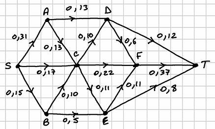
 . The labels are:
  . The path is
  . The flow increase is
  . The saturated arc is
  . Making these amendments, the network looks as follows after this first run:
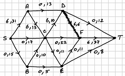
 . The path is
  . The flow increase is
  . The saturated arc is
  . The network looks as follows after this second run:
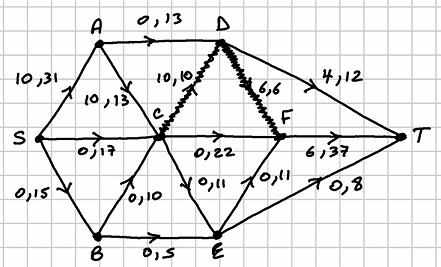
 . The path is
  . The flow increase is
  . The saturated arc is
  . The network looks as follows after this third run:
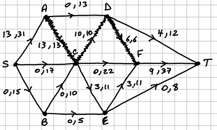
 . The path is
  . The flow increase is
  . The saturated arc is
  . The network looks as follows after this fourth run:
 . The path is
  . The flow increase is
  . The saturated arc is
  . The network looks as follows after this fifth run:
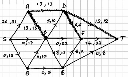
 . The labels are:
  . The path is
  . The flow increase is
  and
and  . The network looks as follows after this sixth run:
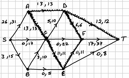
 . The path is
  . The flow increase is
  . The saturated arc is
  . The network looks as follows after this seventh run:
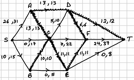
 . The path is
  . The flow increase is
  . The network looks as follows after this eighth run:
 . The labels are:
  . The path is
  . The flow increase is
  . The saturated arc is
  . The network looks as follows after this ninth run:
 . The path is
  . The flow increase is
  . The saturated arc is
  . The network looks as follows after this tenth run:
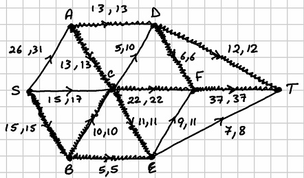
 . The minimum cut is the set of arcs
  which has capacity
  .
.


 ,
,  and
and  joined pairwise by an edge:

 , a heat bath
  , and the total closed system
  ,
,  and
and  respectively so that
 spin configurations with that same energy (i.e., if
  different microstates yielding that same macrostate. Since
  , is a function of
 . Then
  and
and  because we have picked a particular microstate for system

 is the Boltzmann constant.
 is the internal energy of the system and
  is energy added via heat. Using the differential form of the definition of entropy in thermodynamics, namely


 as a relative frequency, the multiplicity of microstates giving energy


 is the average value of the Helmholtz free energy,
  , which is a function of state, i.e., it is a function only of macroscopic thermodynamic variables. The equation
 with
with  . I assumed periodic boundary conditions and the presence of an external magnetic field with parameter
  . The nearest-neighbour Hamiltonian for a particular configuration
  of the
  spins on the four-dimensional hypercube is
 is the spin at site
  on the lattice,
  is the nearest-neighbour interaction energy and
  is the external magnetic field parameter. The partition function assuming thermal equilibrium at a temperature
 . For the computer simulations I used units in which
  and
and  .
. , as a function of the temperature in the range
  to
to  , for a lattice of size
  with
with  ,
,  and
and  . With units in which

 to
to  in multiples of two. I obtained the following results for
  state:
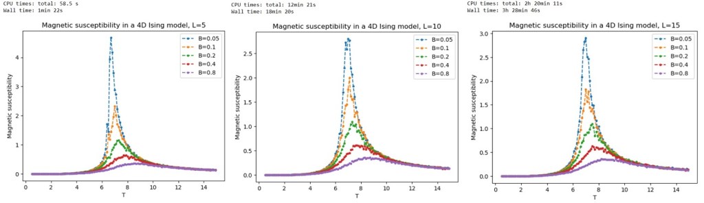
 . Notice also a rapid increase in the CPU time with
  , the CPU time being around one minute for
  .
. 
 at a critical temperature of around
  with Fourier transform
  where
where
 is
is 
 is
is


 so that
  . Then the combined transformation in (2) is obtained as
  which has Fourier transform
 . Therefore, in this case, we have to let
  so that
  . Then the combined transformation in (2) is obtained as
  which has Fourier transform
 parameter in the complex exponential term. This complication is avoided by performing the scaling first before the translation, making this particular ordering of the transformations a little easier to work with in the case of the combined transformation in (2).
 are constants and
  is a standard Wiener process. I used the Euler–Maruyama method with a time step of
  in Python to generate and plot a sample path of this process from
  up to
up to  , setting the initial position as
  and the values
  and
and  . The following picture shows this sample path:
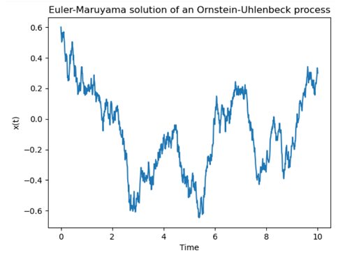
 parameter in the drift term of the SDE, which tends to pull the process back down when
  goes above zero and back up when
 ![\frac{\partial \rho(x, t)}{\partial t} = \gamma \frac{\partial}{\partial x} [x \rho(x, t)] + \frac{\sigma^2}{2}\frac{\partial^2 \rho(x, t)}{\partial x^2} \quad \quad \quad (2)](https://s0.wp.com/latex.php?latex=%5Cfrac%7B%5Cpartial+%5Crho%28x%2C+t%29%7D%7B%5Cpartial+t%7D+%3D+%5Cgamma+%5Cfrac%7B%5Cpartial%7D%7B%5Cpartial+x%7D+%5Bx+%5Crho%28x%2C+t%29%5D+%2B+%5Cfrac%7B%5Csigma%5E2%7D%7B2%7D%5Cfrac%7B%5Cpartial%5E2+%5Crho%28x%2C+t%29%7D%7B%5Cpartial+x%5E2%7D+%5Cquad+%5Cquad+%5Cquad+%282%29+&bg=ffffff&fg=111111&s=1&c=20201002)
 . From (2) we then get
![0 = \gamma \frac{\partial}{\partial x} [x \rho(x, t)] + \frac{\sigma^2}{2}\frac{\partial^2 \rho(x, t)}{\partial x^2}](https://s0.wp.com/latex.php?latex=0+%3D+%5Cgamma+%5Cfrac%7B%5Cpartial%7D%7B%5Cpartial+x%7D+%5Bx+%5Crho%28x%2C+t%29%5D+%2B+%5Cfrac%7B%5Csigma%5E2%7D%7B2%7D%5Cfrac%7B%5Cpartial%5E2+%5Crho%28x%2C+t%29%7D%7B%5Cpartial+x%5E2%7D+&bg=ffffff&fg=111111&s=1&c=20201002)
![= \frac{d}{d x} \bigg[\gamma x \rho(x) + \frac{\sigma^2}{2} \frac{d \rho(x)}{dx} \bigg] \quad \quad \quad \quad (3)](https://s0.wp.com/latex.php?latex=%3D+%5Cfrac%7Bd%7D%7Bd+x%7D+%5Cbigg%5B%5Cgamma+x+%5Crho%28x%29+%2B+%5Cfrac%7B%5Csigma%5E2%7D%7B2%7D+%5Cfrac%7Bd+%5Crho%28x%29%7D%7Bdx%7D+%5Cbigg%5D+%5Cquad+%5Cquad+%5Cquad+%5Cquad+%283%29+&bg=ffffff&fg=111111&s=1&c=20201002)


 from the normalisation condition
 we can rewrite (4) as


 , we have
  and
and  . Using these substitutions together with the expression for


 ,
,  and
and  might be difficult to evaluate manually, but in the case of the Ornstein-Uhlenbeck process these three integrals have simple exact values. For
 and
and  , with limits
  to
to  for
for  and
and  for
for  , and the Cartesian area element
  becoming the polar coordinates area element
  , the double integral becomes
 . It is easily shown that
  , and we can calculate
![= [y \exp(-y^2)]_{-\infty}^{\infty} - \int_{-\infty}^{\infty} y(-2y \exp(-y^2))dy](https://s0.wp.com/latex.php?latex=%3D+%5By+%5Cexp%28-y%5E2%29%5D_%7B-%5Cinfty%7D%5E%7B%5Cinfty%7D+-+%5Cint_%7B-%5Cinfty%7D%5E%7B%5Cinfty%7D+y%28-2y+%5Cexp%28-y%5E2%29%29dy+&bg=ffffff&fg=111111&s=1&c=20201002)


 sample paths of the Ornstein-Uhlenbeck process
  and mean squared distance
  as functions of time together with the corresponding exact values. The plots below show that for sufficiently long times the numerical calculations do indeed fluctuate around the values predicted on the basis of the stationary pdf derived above:
 , derived above from the Fokker-Planck equation. The plot below shows good agreement between the two: