Useful methods in Laplace transform theory

A Laplace transform $L(f)$ of a function $f(t)$ is defined by the equation

$L(f) = \int_0^{\infty} f(t) e^{-pt} dt = F(p) \qquad \qquad \qquad (1)$

The idea is that a Laplace transform takes as an input a function of $t$ , $f(t)$ , and yields as the output a function of $p$ , $F(p)$ .

In many applications of this idea, for example when applying a Laplace transform to the solution of a differential equation, we need to find the inverse of the transform to obtain the required solution. This can often be done by consulting tables of Laplace transforms and their inverses in reference manuals, but we can also invert Laplace transforms using something called the Bromwich integral. I want to explore the latter approach in this note, as it involves the useful trick of solving integrals by converting them to contour integration problems on the complex plane. I also want to record a useful trick for changing the order of integration in double integrals which is employed in the proof of a convolution theorem for Laplace transforms.

Differential equations can be solved using Laplace transforms by finding the transforms of derivatives $y^{\prime} = dy/dt$ , $y^{\prime \prime} = d^2y/dt^2$ , etc. To find $L(y^{\prime})$ , we use the above definition of $L(f)$ and integrate by parts as follows:

$L(y^{\prime}) = \int_0^{\infty} y^{\prime}(t) e^{-pt} dt$

$= \big[e^{-pt} y(t) \big]_0^{\infty} + p\int_0^{\infty} e^{-pt}y(t)dt$

$= -y(0) + pL(y) = pY - y_0 \qquad \qquad \qquad (2)$

where for simplicity we have written $L(y) = Y$ and $y(0) = y_0$ .

To find $L(y^{\prime \prime})$ , we think of $y^{\prime \prime}$ as $(y^{\prime})^{\prime}$ and substitute $y^{\prime}$ for $y$ in (2) to get

$L(y^{\prime \prime}) = pL(y^{\prime}) - y^{\prime}(0)$

$= p(pL(y) - y(0)) - y^{\prime}(0)$

$= p^2 L(y) - py(0) - y^{\prime}(0)$

$= p^2 Y - py_0 - y_0^{\prime} \qquad \qquad \qquad (3)$

Continuing this process, we can also obtain the transforms of higher derivatives. Using these results, we can now solve differential equations. For example, suppose we want to solve

$y^{\prime \prime} + 4y^{\prime} + 4y = t^2 e^{-2t} \qquad \qquad \qquad (4)$

with initial conditions $y_0 = 0$ and $y_0^{\prime} = 0$ . We simply take the Laplace transform of each term in the equation. We get

$p^2 Y - py_0 - y_0^{\prime} + 4pY - 4y_0 + 4Y = L(t^2 e^{-2t}) \qquad \qquad \qquad (5)$

Using the given initial conditions, the left-hand side of (5) reduces to $(p+2)^2 Y$ . We can obtain the Laplace transform on the right-hand side of (5) by consulting a reference table, or by integrating. Following the latter approach, we integrate by parts once to get

$L(t^2e^{-2t}) = \int_0^{\infty} t^2 e^{-2t}e^{-pt}dt = \int_0^{\infty} t^2e^{-(p+2)t}dt = \frac{2}{(p+2)}\int_0^{\infty}t e^{-(p+2)t}dt$

and then integrate by parts again to get

$\int_0^{\infty} t e^{-(p+2)t} = \frac{1}{(p+2)^2}$

Combining these, we get

$L(t^2 e^{-2t}) = \frac{2}{(p+2)^3}$

Alternatively, from standard reference tables we find that

$L(t^k e^{-at}) = \frac{k!}{(p+a)^{k+1}} \qquad \qquad \qquad (6)$

Therefore

$L(t^2 e^{-2t}) = \frac{2}{(p+2)^3}$

Using these results in (5) we get

$(p+2)^2 Y = \frac{2}{(p+2)^3}$

and so

$Y = \frac{2}{(p+2)^5} \qquad \qquad \qquad (7)$

Recall that $Y = L(y)$ , so what we need to do now to solve the problem is to apply an inverse Laplace transform to both sides of (7). This would give

$y = L^{-1}\big(\frac{2}{(p+2)^5}\big) \qquad \qquad \qquad (8)$

We could evaluate the right-hand side of (8) using the formula from the reference table in (6). We see from this formula that we need $k=4$ , $a=2$ , so we can immediately conclude that

$y = L^{-1}\big(\frac{2}{(p+2)^5}\big) = \frac{2t^4e^{-2t}}{4!} = \frac{t^4e^{-2t}}{12} \qquad \qquad \qquad (9)$

This is the required solution to the second-order differential equation in (4) above. What I want to do now is explore the Bromwich integral for Laplace transforms, and use it to confirm the answer in (9) by obtaining the inverse Laplace transform of $\frac{2}{(p+2)^5}$ via the residue theorem from complex analysis.

In the definition of the Laplace transform in (1) above, we now let $p$ be a complex number, say $p = z = x + iy$ . Then the Laplace transform becomes

$F(p) = F(z) = F(x + iy) = \int_0^{\infty} e^{-pt} f(t) dt$

$= \int_0^{\infty} e^{-(x+iy)t} f(t) dt = \int_0^{\infty} e^{-xt} f(t) e^{-iyt} dt \qquad \qquad \qquad (10)$

where $x = \text{Re} \ p > k$ for some real $k$ . [We must have some restriction on $\text{Re} \ p$ to make the integral converge at infinity. The restriction depends on what the function $f(t)$ is, but it is always of the form $\text{Re} \ p > k$ for some real $k$ . To illustrate this idea, consider the case $f(t) = 1$ . Then we have

$\int_0^{\infty} e^{-pt} dt = \big[ -\frac{1}{p}e^{-pt}\big]_0^{\infty} = \frac{1}{p}$

The final equality here holds only for $p > 0$ , because otherwise $e^{-pt}$ would not vanish at the upper limit of the integral. If $p$ is complex, then $\text{Re} \ p > 0$ would be required in this case]. Now, (10) has a form similar to that of a Fourier transform

$g(\alpha) = \frac{1}{2 \pi}\int_{-\infty}^{\infty} f(t) e^{-i \alpha t} dt \qquad \qquad \qquad (11)$

with inverse

$f(t) = \int_{-\infty}^{\infty} g(\alpha) e^{i \alpha t} d \alpha \qquad \qquad \qquad (12)$

$F(p)$ in (10) corresponds to $g(\alpha)$ in (11), and $f(t)$ in (11) corresponds to $\phi(t) = 2 \pi e^{-xt} f(t)$ in (10). Pursuing this analogy with a Fourier transform, the inverse transform for (10), corresponding to (12), would then be

$\phi(t) = \int_{-\infty}^{\infty} F(x + iy) e^{i y t} dy \qquad \qquad \qquad (13)$

Using the definition of $\phi(t)$ , we can write this as

$f(t) = \frac{1}{2 \pi} e^{xt} \int_{-\infty}^{\infty} F(x+iy) e^{i y t} dy$

$= \frac{1}{2 \pi} \int_{-\infty}^{\infty} F(x+iy) e^{(x+iy)t} dy \qquad \qquad \qquad (14)$

for $t > 0$ . Since $x = c$ is a constant in this setup, we have $dz = d(x+iy) = idy$ , so we can write (14) as

$f(t) = \frac{1}{2 \pi i} \int_{c-i\infty}^{c+i\infty} F(x+iy) e^{(x+iy)t} dz$

$= \frac{1}{2 \pi i} \int_{c-i\infty}^{c+i\infty} F(z) e^{zt} dz \qquad \qquad \qquad (15)$

where the notation means that we integrate along a vertical line $x = c$ in the $z$ plane. [This can be any vertical line on which $x = c > k$ as required by the restriction on $\text{Re} \ p$ ]. The integral (15) for the inverse Laplace transform is called the Bromwich integral.

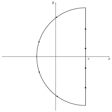
To use (15) to evaluate $f(t)$ for a given $F(p)$ , we exploit the fact that we can evaluate integrals in the complex plane by using the residue theorem. We imagine a contour consisting of a vertical straight line and a semicircle enclosing an area to the left of $x = c$ . We evaluate (15) by using this contour.

We restrict $F(z)$ to be of the form $P(z)/Q(z)$ , with $P(z)$ and $Q(z)$ polynomials, and $Q(z)$ of degree at least one higher than $P(z)$ . The value of the integral around the contour is determined by the singularities lying inside the semicircle, in accordance with the residue theorem. Specifically, the residue theorem says that the integral around the contour equals $2 \pi i$ times the sum of the residues of $F(z)e^{zt}$ at its poles. As the radius of the semicircle goes to infinity, the integral along the straight line becomes an improper integral from $c - i\infty$ to $c+ i\infty$ . However, the integral around the semicircle has the radius appearing to a higher degree in the denominator than in the numerator, so this integral goes to zero as the radius becomes infinite. We are left only with the improper integral along the straight line, and the residue theorem then assures us that this must equal $2 \pi i$ times the sum of the residues of $F(z)e^{zt}$ at its poles . Cancelling the factor $2 \pi i$ from (15), we conclude that

$f(t) = \text{the sum of the residues of } F(z) e^{zt} \text{ at all poles.} \qquad \qquad \qquad (16)$

So, to find $f(t)$ from the Laplace transform $F(p)$ , we simply construct the complex function $F(z)e^{zt}$ , and then sum the residues at all the poles of this constructed function. Note that we must include all poles in (16), i.e., we must choose $x = c$ such that all the poles of $F(z)e^{zt}$ lie inside the contour to the left of the vertical line we are integrating along. To find the residues at each pole, we can use the following rule:

When a function $f(z)$ has a pole of order $n$ at $z_0$ , the residue at this pole can be obtained by multiplying $f(z)$ by $(z - z_0)^n$ , differentiating the result $n-1$ times, dividing by $(n-1)!$ , and evaluating the resulting expression at $z = z_0$ .

We can now apply this approach to find the inverse of the transform

$F(p) = \frac{2}{(p+2)^5}$

We have

$F(z)e^{zt} = \frac{2e^{zt}}{(z+2)^5}$

This has a pole of order 5 at $z = -2$ . Therefore, multiplying by $(z+2)^5$ we get $2e^{zt}$ , differentiating this result $n - 1 = 4$ times we get $2t^4e^{zt}$ , and dividing by $(n - 1)! = 4! = 24$ we get $\frac{t^4 e^{zt}}{12}$ . Finally, evaluating the result at $z = -2$ gives the answer

$f(t) = \frac{t^4e^{-2t}}{12}$

which exactly matches the answer we got in (9) above.

We also have a convolution theorem for Laplace transforms, the proof of which I want to explore here. The convolution theorem says that the Laplace transform of a convolution of functions is the product of the Laplace transforms of the individual functions in the convolution. So, if $g(t)$ and $h(t)$ are functions, and $G(p)$ and $H(p)$ are their corresponding Laplace transforms, then the convolution theorem says

$G(p)H(p) = L\bigg[\int_0^t g(t - \tau)h(\tau) d\tau \bigg] \qquad \qquad \qquad (17)$

where

$(g \ast h)(t) = \int_0^t g(t - \tau)h(\tau) d\tau \qquad \qquad \qquad (18)$

is the convolution of $g$ and $h$ . To prove (17), note that from the definition of a Laplace transform in (1) above we have

$G(p)H(p) = \int_0^{\infty} e^{-pt} g(t) dt \int_0^{\infty} e^{-pt} h(t) dt$

We will now rewrite this by replacing $t$ by different dummy variables of integration so that we can write the product of the two integrals as a double integral. We then have

$G(p)H(p) = \int_0^{\infty} e^{-p \sigma} g(\sigma) d\sigma \int_0^{\infty} e^{-p \tau} h(\tau) d\tau$

$= \int_0^{\infty} \int_0^{\infty} e^{-p(\sigma+\tau)}g(\sigma)h(\tau)d\sigma d\tau \qquad \qquad \qquad (19)$

We now make the change of variables $\sigma + \tau = t$ in the inner integral in (19), i.e., the integral with respect to $\sigma$ , so that $\tau$ is treated as fixed. Then $\sigma = t - \tau$ , $d\sigma = dt$ , and when $\sigma = 0$ we have $t = \tau$ , while when $\sigma = \infty$ we have $t = \infty$ . Then (19) becomes

$G(p)H(p) = \int_{\tau=0}^{\infty} \int_{t=\tau}^{\infty} e^{-pt} g(t-\tau)h(\tau) dt d\tau \qquad \qquad \qquad (20)$

We will now change the order of integration using the following diagrams to interpret what is going on in (20):

From the first diagram, we see that the double integral in (20) is over the area to the right of the diagonal $t = \tau$ line. Within a given strip of width $d\tau$ , the $t$ integral adds up little area elements from the line $t = \tau$ to $t = \infty$ , then the $\tau$ integral sums over the horizontal strips from $\tau = 0$ to $\tau = \infty$ , covering the whole infinite area to the right of the diagonal line. However, we can obtain exactly the same result by considering a vertical strip of width $dt$ as shown in the second diagram. Changing the order of integration and integrating with respect to $\tau$ first, then within the given strip of width $dt$ , the $\tau$ integral adds up little area elements from $\tau = 0$ to the line $\tau = t$ , and then the $t$ integral sums over the vertical strips from $t = 0$ to $t = \infty$ . In doing things this way round, we are working with the double integral

$G(p)H(p) = \int_{t=0}^{\infty} \int_{\tau=0}^{t} e^{-pt}g(t-\tau)h(\tau) d\tau dt$

$= \int_{t=0}^{\infty} e^{-pt} \bigg[\int_{\tau=0}^t g(t-\tau)h(\tau) d\tau \bigg] dt$

$= L\bigg[\int_0^t g(t-\tau)h(\tau) d\tau \bigg] \qquad \qquad \qquad (21)$

where the last step follows from the definition of a Laplace transform in (1) above. As per the construction in the diagrams, the two integrals (20) and (21) must be the same, so the convolution theorem in (17) is proved. The proof is useful in showing how a double infinite integral can be converted into a double integral in which only one of the integrals is improper, and vice versa. I have come across the need for this technique in different contexts.

Useful methods in Laplace transform theory

Published by Dr Christian P. H. Salas

Leave a comment Cancel reply