Some mathematics relating to phonons

A mass connected to a spring and executing simple harmonic motion will oscillate at a natural frequency which is independent of the initial position or velocity of the mass. The particular pattern of vibration at the natural frequency is referred to as the mode of vibration corresponding to that natural frequency. Obviously, there is only one natural frequency and one corresponding mode of vibration for a single mass on a spring. However, a system consisting of two coupled masses connected by springs will, in general, have two distinct natural frequencies (the natural frequencies are often referred to as harmonic frequencies, or simply as harmonics), and two distinct modes of vibration corresponding to these natural frequencies. In general, a system consisting of $N$ masses connected by springs will have $N$ natural frequencies and a distinct mode of vibration for each of these $N$ natural frequencies.

With this in mind, it is interesting to observe that the displacements from equilibrium of an oscillating system of masses connected to springs can be described BOTH in terms of a coupled system of ODEs, AND as an uncoupled system of ODEs, with each independent ODE in the uncoupled system representing a distinct mode of vibration of the original system characterised by a distinct natural frequency. A specific example of this will be given shortly. Amazingly, the same kind of idea also applies to the Hamiltonian of a vibrating lattice of quantum oscillators. The Hamiltonian will initially be expressed in a complicated way involving coupling of the quantum oscillators. However, with some strategic Fourier transforms, the Hamiltonian will be re-expressed in terms of uncoupled entities, each entity representing a distinct mode of vibration of the original lattice characterised by a distinct natural frequency. The transformed Hamiltonian will look exactly the same as the Hamiltonian for an uncoupled set of quantum harmonic oscillators, and quasiparticles called phonons will emerge in this framework as discrete packets of vibrational energy. These phonons are closely analogous to photons as carriers of discrete packets of energy in the context of electromagnetism.

Before considering the case of quantum oscillators in a lattice, it is instructive to explore a specific example of the situation for ODEs describing a simple mass-spring system. Consider two identical pendulums, $A$ and $B$ , connected by a spring whose relaxed length $l$ is exactly equal to the distance between the pendulum bobs.

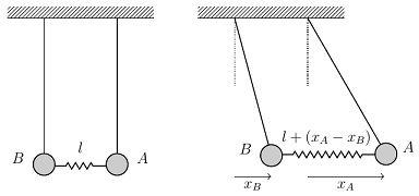
Suppose the system is displaced from equilibrium by moving the pendulums away from their relaxed positions and releasing them. The second picture above shows an arbitrary moment when the displacement of pendulum $A$ is $x_A$ and the displacement of pendulum $B$ is $x_B$ . Since the spring is being stretched by an amount $x_A - x_B$ , the magnitude of the restoring force on $A$ is

$m \omega_0^2 x_A + k (x_A - x_B)$

(i.e., the usual gravitational restoring force for a pendulum, plus the restoring force due to the spring). For $B$ , the magnitude of the restoring force is

$m \omega_0^2 x_B - k (x_A - x_B)$

(the gravitational and spring restoring forces are opposing each other, as can be seen in the sketch above). Therefore using the usual equations $F = m a$ and $F = -kx$ for a spring system, the equations of motion for $A$ and $B$ are

$m \frac{d^2}{dt^2}x_A + m \omega_0^2 x_A + k (x_A - x_B) = 0$

$m \frac{d^2}{dt^2}x_B + m \omega_0^2 x_B - k (x_A - x_B) = 0$

Dividing through by $m$ , and letting $\omega_c^2 = k/m$ , we can write these as

$\frac{d^2}{dt^2}x_A + (\omega_0^2 + \omega_c^2) x_A - \omega_c^2 x_B = 0 \qquad \qquad \qquad (1)$

$\frac{d^2}{dt^2}x_B + (\omega_0^2 + \omega_c^2) x_B - \omega_c^2 x_A = 0 \qquad \qquad \qquad (2)$

These are a pair of coupled ODEs, but we can easily manipulate equations (1) and (2) to obtain two independent ODEs from them. Adding the two equations gives

$\frac{d^2}{dt^2}(x_A + x_B) + \omega_0^2 (x_A + x_B) = 0$

and subtracting (2) from (1) gives

$\frac{d^2}{dt^2}(x_A - x_B) + (\omega_0^2 + 2\omega_c^2) (x_A - x_B) = 0$

Writing $q_1 = x_A + x_B$ and $q_2 = x_A - x_B$ , we can re-express these as

$\frac{d^2}{dt^2}q_1 + \omega_0^2 q_1 = 0 \qquad \qquad \qquad \qquad \qquad (3)$

$\frac{d^2}{dt^2}q_2 + (\omega_0^2 + 2\omega_c^2) q_2 = 0 \qquad \qquad \qquad \ (4)$

These are now two uncoupled ODEs for simple harmonic oscillations, the first one having natural frequency $\omega_0$ and the second one having natural frequency $(\omega_0^2 + 2\omega_c^2)^{1/2}$ . They are independent oscillations because, according to equations (3) and (4), changes in $q_1$ occur independently of changes in $q_2$ , and vice versa. They can be solved independently to get sinusoidal expressions for $q_1$ and $q_2$ . For example, $q_1 = C \cos(\omega_0 t)$ and $q_2 = D \cos( (\omega_0^2 + 2\omega_c^2)^{1/2} t)$ are possible solutions. The transformed equations (3) and (4) represent another way of describing the two normal modes of vibration occurring in the original coupled system (1) and (2), one normal mode having frequency $\omega_0$ , the other having the higher frequency $(\omega_0^2 + 2\omega_c^2)^{1/2}$ .

The present note is concerned with a similar idea at the quantum level, where we imagine $N$ quantum oscillators connected linearly by forces which act like little springs, i.e., a 1-D lattice of quantum oscillators. We want to transform the Hamiltonian for this coupled system into a Hamiltonian which looks like the Hamiltonian for a system of $N$ independent quantum harmonic oscillators. Analogous to the transformed ODE system for the two-mass system considered above, the transformed Hamiltonian will be expressed in terms of the $N$ possible modes of vibration of the original coupled system. The vibration energies in this reformulated Hamiltonian will be seen to consist of discrete `packets’ of energy, $\hbar \omega_k$ , which can be added to, or subtracted from, particular quantum oscillators in the lattice using creation and annihilation operators, just as in the usual quantum harmonic oscillator framework. As stated earlier, these discrete packets of energy can be regarded as particles (or, rather, quasiparticles) analogous to photons in electromagnetism, and they are referred to as phonons in the solid state physics literature. A phonon is thus a quantum of vibrational energy, $\hbar \omega_k$ , needed to move a lattice of coupled quantum oscillators up or down to different vibrational energy levels.

So, we consider a one-dimensional chain of $N$ connected quantum particles, each of mass $m$ , connected by forces which act like springs of unstretched length $a$ and with spring constant $K$ .

The $j$ -th mass is normally at position $R_j = ja$ , but can be displaced slightly by amount $x_j$ . Writing the quantum mechanical momentum and position operators as $\hat{p}_j = - i \hbar \frac{\partial}{\partial x_j}$ and $\hat{x}_j$ respectively, the Hamiltonian operator for the system (a generalisation of the Hamiltonian for a collection of uncoupled quantum oscillators) is

$\hat{H} = \sum_{j=0}^{N-1} \bigg[\frac{\hat{p}_j^{2}}{2m} + \frac{1}{2}K(\hat{x}_{j+1}-\hat{x}_j)^2 \bigg] \qquad \qquad \qquad (5)$

Although this system consists of masses which are strongly coupled to their neighbours by springs, we will show that if the system is perturbed from an initial state where each mass is at position $R_j = ja$ (e.g., by stretching and releasing some of the springs), the vibrations of the 1-D lattice behave as if the system consisted of a set of uncoupled quantum harmonic oscillators. In other words, the Hamiltonian in (5) can be re-expressed in the form

$\hat{H} = \sum_{k=0}^{N-1} \hbar \omega_k \bigg(\hat{a}_k^{\dag} \hat{a}_k + \frac{1}{2}\bigg) \qquad \qquad \qquad (6)$

where $\hbar$ is Planck’s constant, $\omega_k$ is a natural frequency of the system depending on $k$ , and $\hat{a}_k^{\dag}$ and $\hat{a}_k$ are creation and annihilation operators respectively (as in the context of the quantum harmonic oscillator). The subscript $k$ on the creation and annihilation operators reflects the fact that they are only able to act on the $k$ -th oscillator in the system, having no effect on the others. Thus, each oscillator in the system is understood to have its own pair of creation and annihilation operators.

We begin by applying discrete Fourier transforms to the position and momentum operators $\hat{x}_j$ and $\hat{p}_j$ appearing in (5):

$\hat{x}_j = \frac{1}{\sqrt{N}} \sum_{k=0}^{N-1} \hat{x}_k e^{i k j a} \qquad \qquad \qquad \ \ (7)$

$\hat{x}_k = \frac{1}{\sqrt{N}} \sum_{j=0}^{N-1} \hat{x}_j e^{-i k j a} \qquad \qquad \qquad (8)$

$\hat{p}_j = \frac{1}{\sqrt{N}} \sum_{k=0}^{N-1} \hat{p}_k e^{i k j a} \qquad \qquad \qquad \ \ (9)$

$\hat{p}_k = \frac{1}{\sqrt{N}} \sum_{j=0}^{N-1} \hat{p}_j e^{-i k j a} \qquad \qquad \qquad (10)$

We impose periodic boundary conditions, so that

$e^{i k j a} = e^{i k (j + N) a} \qquad \qquad \qquad (11)$

Therefore, we must have

$e^{i k N a} = 1 \qquad \qquad \qquad (12)$

$k = \frac{2 \pi m}{Na} \qquad \qquad \qquad (13)$

where $m$ can take integer values between $0$ and $N-1$ inclusive, i.e., $m$ is in the set of least positive residues of $N$ .

An important observation is that

$\sum_{j=0}^{N-1} e^{i k j a} = N \delta_{k, 0} \qquad \qquad \qquad (14)$

because when $k = 0$ we have a sum of $N$ terms on the left-hand side each equal to $1$ , whereas when $k \neq 0$ we can use the formula for the sum of a geometric progression to write

$\sum_{j=0}^{N-1} e^{i k j a} = \sum_{j=0}^{N-1} (e^{i k a})^j = \frac{(e^{i k a})^N - 1}{e^{i k a} - 1} = 0$

since $(e^{i k a})^N = e^{i 2 \pi m} = 1$ . The result in (14) is used repeatedly in what follows.

Note that (8) is the inverse transform for (7), and (10) is the inverse transform for (9). To see how this works, let us confirm that using (8) in the right-hand side of (7) gives $\hat{x}_j$ . Making the substitution we get

$\frac{1}{\sqrt{N}} \sum_{k=0}^{N-1} \bigg[\frac{1}{\sqrt{N}}\sum_{j^{\prime}=0}^{N-1}\hat{x}_{j^{\prime}} e^{- i k j^{\prime} a}\bigg] e^{i k j a}$

$= \frac{1}{N} \sum_{j^{\prime}=0}^{N-1} \hat{x}_j^{\prime} \bigg[\sum_{k=0}^{N-1} e^{- i k (j^{\prime}-j)a}\bigg]$

$= \frac{1}{N} \sum_{j^{\prime}=0}^{N-1} \hat{x}_{j^{\prime}} N \delta_{(j^{\prime}-j), 0}$

(using (14))

$= \hat{x}_j$

as claimed, since the only non-zero term in the sum in the penultimate line is the one corresponding to $j^{\prime} = j$ . Thus, $\hat{x}_k$ in (8) is the inverse operator of $\hat{x}_j$ in (7), and likewise $\hat{p}_k$ in (10) is the inverse operator of $\hat{p}_j$ in (9).

Next, we observe that for the usual operators in (7) and (9) we have the commutation relations

$[\hat{x}_j, \hat{p}_{j^{\prime}}] = i \hbar \delta_{j, j^{\prime}} \qquad \qquad \qquad (15)$

The inverse transforms in (8) and (10) then imply that we have the following commutation relations for the inverse operators:

$[\hat{x}_k, \hat{p}_{k^{\prime}}] = i \hbar \delta_{k, -k^{\prime}} \qquad \qquad \qquad (16)$

To see this, observe that we have

$[\hat{x}_k, \hat{p}_{k^{\prime}}] = \frac{1}{\sqrt{N}} \sum_{j=0}^{N-1} \hat{x}_j e^{- i k j a} \cdot \frac{1}{\sqrt{N}} \sum_{j^{\prime}=0}^{N-1} \hat{p}_{j^{\prime}} e^{-i k^{\prime} j^{\prime} a}$

$- \frac{1}{\sqrt{N}} \sum_{j^{\prime}=0}^{N-1} \hat{p}_{j^{\prime}} e^{- i k^{\prime} j^{\prime} a} \cdot \frac{1}{\sqrt{N}} \sum_{j=0}^{N-1} \hat{x}_j e^{- i k j a}$

$= \frac{1}{N} \sum_{j=0}^{N-1} \sum_{j^{\prime}=0}^{N-1} e^{-i k j a} e^{- i k^{\prime} j^{\prime} a} [\hat{x}_j, \hat{p}_{j^{\prime}}]$

$= \frac{1}{N} i \hbar \sum_{j = 0}^{N-1} e^{- i (k + k^{\prime}) j a}$

(using (15))

$= \frac{1}{N} i \hbar N \delta_{k, -k^{\prime}}$

(using (14))

$= i \hbar \delta_{k, -k^{\prime}}$

as claimed.

With these results we are now in a position to work out the terms in the Hamiltonian in (5) above in terms of the inverse operators $\hat{p}_k$ and $\hat{x}_k$ . First, using (9), we have

$\sum_{j=0}^{N-1} \hat{p}_j^2$

$= \sum_{j=0}^{N-1} \bigg(\frac{1}{\sqrt{N}}\sum_{k=0}^{N-1}\hat{p}_k e^{i k j a}\bigg) \bigg(\frac{1}{\sqrt{N}}\sum_{k^{\prime}=0}^{N-1}\hat{p}_{k^{\prime}} e^{i k^{\prime} j a}\bigg)$

$= \frac{1}{N} \sum_{j=0}^{N-1} \sum_{k=0}^{N-1} \sum_{k^{\prime}=0}^{N-1} \hat{p}_k \hat{p}_{k^{\prime}} e^{i (k + k^{\prime}) j a}$

$= \frac{1}{N} \sum_{k=0}^{N-1} \sum_{k^{\prime}=0}^{N-1} \hat{p}_k \hat{p}_{k^{\prime}} \bigg(\sum_{j=0}^{N-1}e^{i (k + k^{\prime}) j a}\bigg)$

(carrying out the spatial sum)

$= \frac{1}{N} \sum_{k=0}^{N-1} \sum_{k^{\prime}=0}^{N-1} \hat{p}_k \hat{p}_{k^{\prime}} N \delta_{k, -k^{\prime}}$

(using (14))

$= \sum_{k=0}^{N-1} \sum_{k^{\prime}=0}^{N-1} \hat{p}_k \hat{p}_{k^{\prime}} \delta_{k, -k^{\prime}}$

$= \sum_{k=0}^{N-1} \hat{p}_k \hat{p}_{-k} \qquad \qquad \qquad (17)$

where in the last step we used the Kronecker delta to carry out one of the momentum sums. This has the effect of setting $k^{\prime} = -k$ (because any term not satisfying this will disappear), leaving us with a sum over a single index.

Next, using (7), we have

$\hat{x}_{j+1} = \frac{1}{\sqrt{N}} \sum_{k=0}^{N-1} \hat{x}_k e^{i k (j+1)a}$

$= \frac{1}{\sqrt{N}} \sum_{k=0}^{N-1} \hat{x}_k e^{i k j a} e^{i k a}$

Subtracting (7) from this we get

$\hat{x}_{j+1} - \hat{x}_j = \frac{1}{\sqrt{N}} \sum_{k=0}^{N-1} \hat{x}_k e^{i k j a}(e^{i k a} - 1)$

Using this to deal with the other terms in the Hamiltonian in (5) we get

$\sum_{j=0}^{N-1} (\hat{x}_{j+1} - \hat{x}_j)^2$

$= \frac{1}{N} \sum_{j=0}^{N-1} \sum_{k=0}^{N-1} \sum_{k^{\prime}=0}^{N-1} \hat{x}_k \hat{x}_{k^{\prime}} e^{i (k + k^{\prime}) j a} (e^{i k a} - 1)(e^{i k^{\prime} a} - 1)$

$= \frac{1}{N} \sum_{k=0}^{N-1} \sum_{k^{\prime}=0}^{N-1} \hat{x}_k \hat{x}_{k^{\prime}} (e^{i k a} - 1)(e^{i k^{\prime} a} - 1)\bigg(\sum_{j=0}^{N-1}e^{i (k + k^{\prime}) j a}\bigg)$

$= \frac{1}{N} \sum_{k=0}^{N-1} \sum_{k^{\prime}=0}^{N-1} \hat{x}_k \hat{x}_{k^{\prime}} (e^{i k a} - 1)(e^{i k^{\prime} a} - 1)N\delta_{k, -k^{\prime}}$

$= \sum_{k=0}^{N-1} \hat{x}_k \hat{x}_{-k} (e^{i k a} - 1)(e^{- i k a} - 1)$

$= \sum_{k=0}^{N-1} \hat{x}_k \hat{x}_{-k} (1 - e^{i k a} - e^{- i k a} + 1)$

$= \sum_{k=0}^{N-1} \hat{x}_k \hat{x}_{-k} \big(1 - \cos(ka) - i \sin(ka) - \cos(ka) + i \sin(ka) + 1\big)$

$= \sum_{k=0}^{N-1} \hat{x}_k \hat{x}_{-k} 2 \big(1 - \cos(ka) \big)$

$= \sum_{k=0}^{N-1} \hat{x}_k \hat{x}_{-k} \big(4 \sin^2\big(\frac{ka}{2}\big)\big) \qquad \qquad \qquad (18)$

(using the result $1 - \cos(\theta) = 2\sin^2(\theta/2)$ ).

Using (17) and (18), we can rewrite the Hamiltonian in (5) as

$\hat{H} = \sum_{k=0}^{N-1} \bigg[\frac{1}{2m} \hat{p}_k \hat{p}_{-k} + \frac{1}{2} m \omega_k^2 \hat{x}_k \hat{x}_{-k} \bigg] \qquad \qquad \qquad (19)$

where $\omega_k^2 \equiv 4(K/m) \sin^2 (ka/2)$ .

Next, we observe from (10) that the Hermitian conjugate of $\hat{p}_k$ is given by

$\hat{p}_k^{\dag} = \frac{1}{\sqrt{N}} \sum_{j=0}^{N-1} \hat{p}_j^{\dag} e^{i k j a}$

But since $\hat{p}_j$ is Hermitian, we have $\hat{p}_j^{\dag} = \hat{p}_j$ . Therefore

$\hat{p}_k^{\dag} = \frac{1}{\sqrt{N}} \sum_{j=0}^{N-1} \hat{p}_j e^{i k j a} = \hat{p}_{-k} \qquad \qquad \qquad (20)$

A similar argument using (8) shows that

$\hat{x}_k^{\dag} = \hat{x}_{-k} \qquad \qquad \qquad (21)$

[Formally, the adjoint of an operator $A$ is defined by $\langle \psi, A \phi \rangle = \langle A^{\dag} \psi, \phi \rangle$ . In the case of a Hermitian operator, we have $\langle \psi, A \phi \rangle = \langle A \psi, \phi \rangle$ . Therefore, $A^{\dag} = A$ . This guarantees that the operator has real eigenvalues. In our case, by working out the inner products $\langle \psi, \hat{p}_j \phi \rangle$ and $\langle \hat{p}_j \psi, \phi \rangle$ , for example, we would find that they are equal, confirming that $\hat{p}_j^{\dag} = \hat{p}_j$ ].

Using these results with (16), we can write down the commutation relation between $\hat{x}_k$ and $\hat{p}_k^{\dag}$ as

$[\hat{x}_k, \hat{p}_{k^{\prime}}^{\dag}] = [\hat{x}_k, \hat{p}_{-k^{\prime}}] = i \hbar \delta_{k, k^{\prime}} \qquad \qquad \qquad (22)$

We can also write down the creation and annihilation operators (cf. the quantum harmonic oscillator) as

$\hat{a}_k = \sqrt{\frac{m \omega_k}{2 \hbar}} \big(\hat{x}_k + \frac{i}{m \omega_k} \hat{p}_k\big) \qquad \qquad \qquad \ \ \ \ (23)$

$\hat{a}_k^{\dag} = \sqrt{\frac{m \omega_k}{2 \hbar}} \big(\hat{x}_{-k} - \frac{i}{m \omega_k} \hat{p}_{-k}\big) \qquad \qquad \qquad (24)$

It is easy to show that these satisfy the commutation relations

$[\hat{a}_k^{\dag}, \hat{a}_{k^{\prime}}^{\dag}] = 0 \qquad \qquad \qquad \ \ \ (25)$

$[\hat{a}_k, \hat{a}_{k^{\prime}}] = 0 \qquad \qquad \qquad \ \ \ (26)$

$[\hat{a}_k, \hat{a}_{k^{\prime}}^{\dag}] = \delta_{k, k^{\prime}} \qquad \qquad \qquad (27)$

Therefore, creation and annihilation operators with subscript $k$ can only act on an oscillator corresponding to the same wave vector $k$ . When they try to act on an oscillator corresponding to a different wave vector, they commute, so they are unable to have any effect. To demonstrate (27) in the case $k^{\prime} = k$ , we have

$[\hat{a}_k, \hat{a}_k^{\dag}] = \hat{a}_k \hat{a}_k^{\dag} - \hat{a}_k^{\dag} \hat{a}_k$

$= \frac{m \omega_k}{2 \hbar} \bigg[\big(\hat{x}_k + \frac{i}{m \omega_k} \hat{p}_k\big) \big(\hat{x}_{-k} - \frac{i}{m \omega_k} \hat{p}_{-k}\big) - \big(\hat{x}_{-k} - \frac{i}{m \omega_k} \hat{p}_{-k}\big) \big(\hat{x}_k + \frac{i}{m \omega_k} \hat{p}_k\big)\bigg]$

$= \frac{m \omega_k}{2 \hbar} \bigg[-\frac{i}{m \omega_k}\hat{x}_k\hat{p}_{-k} + \frac{i}{m\omega_k}\hat{p}_k\hat{x}_{-k} - \frac{i}{m\omega_k}\hat{x}_{-k}\hat{p}_k + \frac{i}{m\omega_k}\hat{p}_{-k}\hat{x}_k\bigg]$

$= \frac{m \omega_k}{2 \hbar} \bigg[-\frac{i}{m\omega_k}[\hat{x}_k, \hat{p}_{-k}] + \frac{i}{m\omega_k}[\hat{p}_k, \hat{x}_{-k}]\bigg]$

$= \frac{m \omega_k}{2 \hbar} \bigg[-\frac{i}{m\omega_k}(i \hbar) + \frac{i}{m\omega_k}(-i\hbar)\bigg]$

$= 1$

as required.

We can invert equations (23) and (24). From (24) we get

$\hat{a}_{-k}^{\dag} = \sqrt{\frac{m \omega_k}{2\hbar}}\big(\hat{x}_k - \frac{i}{m\omega_k}\hat{p}_k\big)$

$\hat{x}_k = \sqrt{\frac{2\hbar}{m\omega_k}}\hat{a}_{-k}^{\dag} + \frac{i}{m\omega_k}\hat{p}_k \qquad \qquad \qquad (28)$

Using (28) to substitute for $\hat{x}_k$ in (23) we get, with some easy manipulations,

$\hat{p}_k = -i\sqrt{\frac{m\hbar\omega_k}{2}}\big(\hat{a}_k - \hat{a}_{-k}^{\dag}\big) \qquad \qquad \qquad (29)$

And using (29) to substitute for $\hat{p}_k$ in (28) we get

$\hat{x}_k = \sqrt{\frac{\hbar}{2m\omega_k}}\big(\hat{a}_{-k}^{\dag} + \hat{a}_k\big) \qquad \qquad \qquad (30)$

Therefore, using (29), we deduce

$\frac{1}{2m}\hat{p}_k\hat{p}_{-k}$

$= \frac{1}{2m}\bigg( -i\sqrt{\frac{m\hbar\omega_k}{2}}\big(\hat{a}_k - \hat{a}_{-k}^{\dag}\big) \bigg)\bigg( -i\sqrt{\frac{m\hbar\omega_k}{2}}\big(\hat{a}_{-k} - \hat{a}_k^{\dag}\big) \bigg)$

$= -\big(\frac{\hbar \omega_k}{4}\big)\big(\hat{a}_k \hat{a}_{-k} - \hat{a}_k \hat{a}_k^{\dag} - \hat{a}_{-k}^{\dag} \hat{a}_{-k} + \hat{a}_{-k}^{\dag} \hat{a}_k^{\dag}\big) \qquad \qquad \qquad (31)$

and, similarly, using (30) we deduce

$\frac{1}{2}m\omega_k^2 \hat{x}_k \hat{x}_{-k}$

$= \frac{1}{2}m\omega_k^2 \bigg( \sqrt{\frac{\hbar}{2m\omega_k}}\big(\hat{a}_{-k}^{\dag} + \hat{a}_k\big) \bigg)\bigg( \sqrt{\frac{\hbar}{2m\omega_k}}\big(\hat{a}_{k}^{\dag} + \hat{a}_{-k}\big) \bigg)$

$= \big(\frac{\hbar \omega_k}{4}\big) \big(\hat{a}_k \hat{a}_{-k} + \hat{a}_k \hat{a}_k^{\dag} + \hat{a}_{-k}^{\dag} \hat{a}_{-k} + \hat{a}_{-k}^{\dag} \hat{a}_k^{\dag}\big) \qquad \qquad \qquad (32)$

Adding (31) and (32) we get

$\frac{\hbar \omega_k}{2}\big(\hat{a}_k\hat{a}_k^{\dag} + \hat{a}_{-k}^{\dag} \hat{a}_{-k}\big) \qquad \qquad \qquad (33)$

Therefore the Hamiltonian in (19) becomes

$\hat{H} = \sum_{k=0}^{N-1} \bigg[\frac{\hbar \omega_k}{2} \big(\hat{a}_k\hat{a}_k^{\dag} + \hat{a}_{-k}^{\dag} \hat{a}_{-k}\big) \bigg] \qquad \qquad \qquad (34)$

But, by inspection, $\hat{a}_{-k}^{\dag} \hat{a}_{-k}$ and $\hat{a}_{k}^{\dag} \hat{a}_{k}$ are the same operators, just expressed with different indices. Therefore, re-indexing this term in the Hamiltonian in (34) we get

$\hat{H} = \sum_{k=0}^{N-1} \bigg[\frac{\hbar \omega_k}{2} \big(\hat{a}_k\hat{a}_k^{\dag} + \hat{a}_{k}^{\dag} \hat{a}_{k}\big) \bigg] \qquad \qquad \qquad (35)$

Finally, using the commutator in (27) with $k^{\prime} = k$ , we have

$\hat{a}_k \hat{a}_k^{\dag} = 1 + \hat{a}_k^{\dag} \hat{a}_k$

Therefore, the Hamiltonian in (35) can be written as

$\hat{H} = \sum_{k=0}^{N-1} \bigg[\hbar \omega_k \bigg(\hat{a}_{k}^{\dag} \hat{a}_{k} + \frac{1}{2}\bigg) \bigg] \qquad \qquad \qquad (36)$

which is the same as (6). This result shows that the Hamiltonian for a linear chain of coupled quantum oscillators can be expressed in terms of modes of vibration which behave like independent and uncoupled quantum harmonic oscillators. The $k$ -th mode of vibration can accept increments to its energy in integer multiples of a basic quantum of energy, $\hbar \omega_k$ . As in the standard quantum harmonic oscillator model, these quanta of energy behave like particles, and we call these quanta phonons in the present context.

Some mathematics relating to phonons

Published by Dr Christian P. H. Salas

Leave a comment Cancel reply