Study of a Lagrangian function approach to analysing raindrop growth

In this note, I study a constrained maximisation approach seeking to clarify the growth history of microscopic water droplets which undergo runaway aggregation to become raindrops. Using this approach, and the setup outlined in a previous note about a 2016 paper in Physical Review Letters on the large deviation analysis of rapid-onset rain showers (referred to as MW2016 herein), an expression for the total time for runaway growth is easily obtained in terms of the mean inter-collision times $\tau_n$ . This expression seems to be related in some way to the expression for $\tau$ in MW2016, which was derived from large deviation analysis. The purpose of the present note is to try to further clarify the links with some of the results in MW2016. In order to achieve this, I employed a Lagrangian function approach to the constrained maximisation problem as follows.

A Lagrangian function approach

Let the random variable $T$ , representing the total time required for a droplet to undergo runaway growth, be defined as in the previous note mentioned above, that is,

$T = \sum_{n=1}^{\mathcal{N}} t_n$

where the inter-collision times $t_n$ are independent exponentially distributed random variables with mean $\tau_n = 1/R_n$ . The parameter $\mathcal{N}$ is a given total number of water particle collisions required for runaway growth of a raindrop.

Consider also a fixed time interval $[0, \tau]$ , where $\tau \equiv \bar{T}/\langle T \rangle$ , and $\bar{T}$ is a number in the small-value tail of the distribution of $T$ , to be treated as an exogenous parameter in the forthcoming analysis. We partition the interval $[0, \tau]$ into $\mathcal{N}$ subintervals, each of length $\hat{t}_n$ , so that

$\tau = \sum_{n=1}^{\mathcal{N}} \hat{t}_n \qquad \qquad \qquad \qquad \qquad (1)$

Then on the basis of the exponential distributions of the inter-collision times $t_n$ , we have the following joint cumulative distribution function for the inter-collision times:

$P(t_1 \leq \hat{t_1}, t_2 \leq \hat{t}_2, \ldots, t_{\mathcal{N}} \leq \hat{t}_{\mathcal{N}}) = \prod_{n=1}^{\mathcal{N}} (1 - \exp(-\hat{t}_n/\tau_n)) \qquad \qquad \qquad \qquad \qquad (2)$

In the constrained maximisation approach, we seek to choose the inter-collision time parameters $\hat{t}_n$ to maximise the joint cumulative distribution function in (2), subject to the constraint represented by (1). Since logarithms are monotone increasing functions, we can obtain the same results by maximising the natural logarithm of (2) subject to (1). The Lagrangian function for this constrained maximisation problem can then be written as

$\mathcal{L} = \sum_{n=1}^{\mathcal{N}} \ln(1 - \exp(-\hat{t}_n/\tau_n)) + k \bigg(\tau - \sum_{n=1}^{\mathcal{N}} \hat{t}_n \bigg) \qquad \qquad \qquad \qquad \qquad (3)$

where I have used the symbol $k$ to denote the Lagrange multiplier, since this will turn out to be closely linked to the Laplace transform parameter $k$ in the large deviation analysis in MW2016. First-order conditions for a maximum are

$\frac{\partial \mathcal{L}}{\partial \hat{t}_n} = \frac{\frac{1}{\tau_n}\exp(-\hat{t}_n/\tau_n)}{1 - \exp(-\hat{t}_n/\tau_n)} - k = 0 \qquad \qquad \qquad \qquad \qquad (4)$

for $n = 1, \ldots, \mathcal{N}$ , and

$\frac{\partial \mathcal{L}}{\partial k} = \tau - \sum_{n=1}^{\mathcal{N}} \hat{t}_n = 0 \qquad \qquad \qquad \qquad \qquad (5)$

Solving (4) gives

$\hat{t}_n^{\ast} = \tau_n \ln\bigg(1 + \frac{1}{k^{\ast} \tau_n}\bigg) \qquad \qquad \qquad \qquad \qquad (6)$

and putting this into (5) gives

$\tau = \sum_{n=1}^{\mathcal{N}} \tau_n \ln\bigg(1 + \frac{1}{k^{\ast} \tau_n}\bigg) \qquad \qquad \qquad \qquad \qquad (7)$

where $\hat{t}_n^{\ast}$ and $k^{\ast}$ denote the optimised values of $\hat{t}_n$ and $k$ respectively, given the value of the parameter $\tau$ . We can now put this structure to work and clarify its links with runaway growth of raindrops and with the large deviation analysis in MW2016.

First, we obtain an intuitively appealing interpretation of the optimised Lagrange multiplier $k^{\ast}$ by solving (6) for $k^{\ast}$ in the case $n=1$ . Noting that $\tau_1=1$ , this gives

$k^{\ast} = \frac{1}{\exp(\hat{t}_1^{\ast}) - 1} \qquad \qquad \qquad \qquad \qquad (8)$

Therefore, for small $\tau$ and $\hat{t}_1^{\ast} \ll 1$ , we have $k^{\ast} \approx 1/\hat{t}_1^{\ast}$ , so the maximised Lagrange multiplier can be interpreted as the reciprocal of the first monomer collision time in the runaway growth process. Thus, $k^{\ast}$ can be expected to be very large in scenarios in which $\hat{t}_1^{\ast}$ is very small.

Next, put the expressions for $\hat{t}_n^{\ast}$ in (6) into the Lagrangian function in (3), to obtain the following expression for the maximised value of the Lagrangian as a function only of $k^{\ast}$ :

$\mathcal{L}^{\ast} = - \bigg \{\sum_{n=1}^{\mathcal{N}} \ln(1 + k^{\ast} \tau_n) - k^{\ast} \tau \bigg \} - \sum_{n=1}^{\mathcal{N}} k^{\ast} \tau_n \ln\bigg(1 + \frac{1}{k^{\ast} \tau_n}\bigg) \qquad \qquad \qquad \qquad \qquad (9)$

In the regime of a small $\tau$ , $\hat{t}_1^{\ast} \ll 1$ , and $k^{\ast} \gg 1$ , the second term on the right-hand side of (9) would converge to the constant $\mathcal{N}$ , and we recognise the first bracketed term on the right-hand side of (9) as being of the same form as the entropy function in MW2016. Therefore, as $\tau \rightarrow 0$ , and $k^{\ast} \rightarrow \infty$ , we obtain the result

$\mathcal{L}^{\ast \prime}(k^{\ast}) \sim -J^{\prime}(k^{\ast}) = 0 \qquad \qquad \qquad \qquad \qquad (10)$

which then leads to the same function $\tau(k^{\ast})$ as the one derived from the large deviation analysis in MW2016. However, in the regime of larger values of $\tau$ for which $k^{\ast}$ is not large, the correct expression for $\tau(k^{\ast})$ is (7) above, obtained when the second term on the right-hand side of (9) is no longer negligible when calculating $\mathcal{L}^{\ast \prime}(k^{\ast})$ .

A geometric understanding of the relationship between the two approaches can also be obtained by recognising a probabilistic connection between them. We can extend to our $\mathcal{N}$ -dimensional case an elementary result in probability theory relating the cumulative distribution function of a sum of random variables to the joint density function of those same random variables by writing

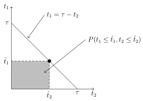
$P\bigg(\sum_{n=1}^{\mathcal{N}} t_n \leq \tau\bigg)$

$= \int_0^{\tau} \cdots \int_0^{\tau - \sum_{n=2}^{\mathcal{N}} t_n} \{f_1(t_1)f_2(t_2) \cdots f_{\mathcal{N}}(t_{\mathcal{N}})\} \ dt_1 \cdots dt_{\mathcal{N}} \qquad \qquad \qquad \qquad \qquad (11)$

Given that the inter-collision times are independent, the integrand on the right-hand side of (11) is the joint probability density function of the inter-collision times $t_1, t_2, \ldots, t_{\mathcal{N}}$ , which also appear in the sum in the cumulative distribution function on the left-hand side of (11). To clarify the situation geometrically, consider the two-dimensional case depicted in the following diagram.

In two dimensions, the probability represented by (11) is the probability mass in the shaded region bounded by the coordinate axes and the diagonal line.

The link between this framework, and the exponential function of the entropy function $J(\tau)$ that appears in the large deviation analysis in MW2016, $\exp(-J(\tau))$ , is that the latter has the probabilistic interpretation that it is the smallest possible upper bound of the probability that the random sum of inter-collision times is greater than $\tau$ when using the form of Markov’s inequality in the Cramér-Chernoff bounding method (see my previous note about this}. Therefore, negating this relationship, we have

$P\bigg(\sum_{n=1}^{\mathcal{N}} t_n \leq \tau\bigg) \geq 1 - \exp(-J(\tau)) \qquad \qquad \qquad \qquad \qquad (12)$

So, by using the Fenchel-Legendre transform $J(\tau)$ , the approach in MW2016 is implicitly maximising the lower bound of the probability that the sum of inter-collision times is no greater than $\tau$ in (12), and $1 - \exp(-J(\tau))$ then constitutes an approximation of the probability mass represented in two dimensions by the shaded region in the diagram above.

The link with the constrained maximisation approach is that here we are approximating the probability as represented by the right-hand side of (11) by choosing the parameters $\hat{t}_n$ to obtain the maximum of the joint cumulative distribution function of the inter-collision times. In the two-dimensional case, this corresponds to choosing a point on the diagonal line in the diagram below in order to maximise the probability mass in the rectangular region.

The upshot, then, is that the multi-dimensional analogue of maximising the probability mass in the rectangular region in the second diagram above by choosing the $\hat{t}_n$ optimally, and the multi-dimensional analogue of approximating the probability mass in the entire region below the diagonal line using the entropy function $J(\tau)$ in $1 - \exp(-J(\tau))$ , both converge to the same result in the small $\tau$ and small $\hat{t}_1^{\ast}$ regime for which $k^{\ast} \gg 1$ . The two approaches deviate from each other in the large $\tau$ /small $k^{\ast}$ regime due to the logarithmic correction term in (9).

Finally in this section, I briefly record some numerical results from using MAPLE to implement equations (6) and (7). Substituting equation (8) into (6) and (7), and using $\tau_n = 1/n^2$ , we obtain

$\hat{t}_n^{\ast} = \frac{1}{n^2} \ln\big(1 + n^2 (\exp(\hat{t}_1^{\ast})-1)\big) \qquad \qquad \qquad \qquad \qquad (13)$

for $n = 1, \ldots, \mathcal{N}$ , and

$\tau = \sum_{n=1}^{\mathcal{N}} \frac{1}{n^2} \ln\big(1 + n^2 (\exp(\hat{t}_1^{\ast})-1)\big) \qquad \qquad \qquad \qquad \qquad (14)$

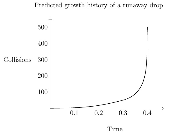
Thus, given a value for $\tau$ , the maximum-likelihood time $\hat{t}_1^{\ast}$ for the first monomer collision can be computed from (14), and then this value can be used to determine $\hat{t}_n^{\ast}$ for each $n = 2, \dots, \mathcal{N}$ via (13). A plot of the number of collisions versus time, i.e., the growth history of a runaway drop, can then be obtained by plotting the points with coordinates $\big(\big \{\sum_{n=1}^{m}\hat{t}_n^{\ast}\big \}, m \big)$ for $m = 1, 2, \dots$ . For example, a MAPLE computation with values $\tau = 0.4136$ and $\mathcal{N} = 10,000$ , inspired by some FORTRAN simulations, produced a first monomer collision time $\hat{t}_1^{\ast} = 0.018$ and a growth history plot like the one shown in the following diagram. The shape of this plot is typical of the runaway growth plots also produced by some physical FORTRAN simulations (not shown here).

Interpretation as constrained maximum likelihood

At first sight, the constrained maximisation approach in this section looks different from a traditional maximum likelihood calculation because the objective function (2) involves the cumulative distribution functions of the inter-collision times rather than probability densities. However, the approach can in fact be interpreted as a constrained maximum likelihood problem with left-censoring of the inter-collision times. Censored data arise frequently in econometrics and other statistical disciplines when some values of a variable of interest fall within a certain range that renders them unobservable. Such observations are then all reported in a collected data set as having a value equal to the boundary of the unobservable range. The objective functions used for maximum likelihood estimation in these settings will necessarily involve the cumulative distribution functions of the variables of interest, because probability densities cannot be evaluated at single points for censored data. See, for example, Gentleman, R., Geyer, C., 1994, Maximum likelihood for interval censored data: consistency and computation, Biometrika, Vol. 81, No. 3, pp. 618-623, and also pages 761-768 in Greene, W., 2003, Econometric Analysis, Fifth Edition, Prentice-Hall International (UK) Limited, London.

In our constrained maximisation calculation in this section, what we are essentially saying is this: we cannot observe the actual inter-collision times $t_n$ , so assume that all we know is that the inter-collision times $t_n$ are below some threshold values $\hat{t}_n$ . (In econometrics, this would be referred to as left-censoring). Then given the exponential distributions for the inter-collision times, what is the most likely sequence of threshold values $\hat{t}_n$ for a runaway raindrop? It is important to understand, however, that we are not addressing this question here in a statistical way with observed data. Maximum likelihood estimation has some well known disadvantages in statistical contexts, particularly when the number of parameters to be estimated is large. Distortions can arise in maximum likelihood estimation involving the gamma distribution, for example, due to unwanted correlations between parameter estimates. See, e.g., Bowman, K., Shenton, L., 2002, Problems with maximum likelihood estimation and the 3 parameter gamma distribution, Journal of Statistical Computation and Simulation, 72:5 pp. 391-401. However, we are not doing statistical maximum likelihood here, in the sense that we are not using observed data to estimate parameters. We are doing mathematical maximum likelihood, just using the functional forms of the probability distributions of the runaway drops. In this context, the statistical problems with the maximum likelihood method are irrelevant, so the approach here actually represents a potentially powerful mathematical method for analysing raindrop histories that can also be applied in the context of other problems. It also has direct links to the entropy functions of large deviation theory, as was demonstrated using the Lagrangian function approach above.

Study of a Lagrangian function approach to analysing raindrop growth

Published by Dr Christian P. H. Salas

Leave a comment Cancel reply