A spline approximation scheme for large deviation theory problems

In this note, I develop and implement a spline function approximation scheme that can quickly generate accurate benchmark solutions for large deviation theory problems. To my knowledge, spline function approximation methods have not been applied before in the context of large deviation theory. This note shows that such methods can be efficient and effective even when it is computationally difficult or impossible to obtain the required numerical results in other ways.

In fact, the effort in this note was initially motivated by computational difficulties encountered while trying to obtain fine-grained sets of numerical values for the large deviation functions in a 2016 paper in Physical Review Letters (outlined in a previous note) about the large deviation analysis of rapid-onset rain showers. This paper will be referred to as MW2016 herein. It is desirable to carry out such computations using sophisticated mathematical software systems such as MAPLE, which come with many built-in features that can make the necessary programming convenient and transparent. However, attempts to compute fine-grained exact function values for the cumulant generating function and its derivatives proved to be difficult and time consuming in MAPLE. Carrying out these computations for the case $\gamma=2$ took hours and it was even more time consuming to obtain the necessary fine-grained exact function values for the case $\gamma = 4/3$ . In view of these difficulties, it seemed desirable to attempt to develop a new numerical solution system for large deviation problems that would enable accurate numerical results to be produced in MAPLE, using only the simplest mathematical functions. This note reports my experiments with one way of achieving this using cubic spline functions.

A closer look at the cumulant generating function

For what follows, assume the same simple power law collision rates $R_n$ as in MW2016, with the normalisations $R_1 =1$ and $\langle T \rangle = 1$ . Also assume a given collision rate parameter $\gamma \in [4/3,2]$ , and that $k > 0$ . The cumulant generating function in equation [14] in MW2016 is then a smooth, strictly concave function in both $k$ and $N$ . To see this, write it as

$\lambda(N, k; \gamma) = \sum_{n=1}^N \ln\bigg(1 + \frac{k}{n^{\gamma}}\bigg) \qquad \qquad \qquad \qquad \qquad (1)$

The first two partial derivatives with respect to $k$ are

$\frac{\partial \lambda(N, k;\gamma)}{\partial k} = \sum_{n=1}^N \frac{1}{n^{\gamma} + k} > 0 \qquad \qquad \qquad \qquad \qquad (2)$

and

$\frac{\partial^2 \lambda(N, k;\gamma)}{\partial k^2} = - \sum_{n=1}^N \frac{1}{(n^{\gamma} + k)^2} < 0 \qquad \qquad \qquad \qquad \qquad (3)$

which confirms strict concavity with respect to $k$ . To find the partials with respect to $N$ , we can use the Euler-Maclaurin formula to express (1) as

$\lambda(N, k; \gamma) = \int_1^N dn f(n) + \frac{1}{2} \big(f(1) + f(N)\big)$

$- \sum_{m=1}^{\mathcal{M}} \frac{B_{2m}}{(2m)!} \big(f^{(2m-1)}(1) - f^{(2m-1)}(N)\big) + R_{\mathcal{M}+1} \qquad \qquad \qquad \qquad \qquad (4)$

where $f(n) = \ln\big(1+\frac{k}{n^{\gamma}}\big)$ , $B_{2m}$ are the even-indexed Bernoulli numbers, and $R_{\mathcal{M}+1}$ is a remainder term. Numerical experiments with MAPLE indicate that only the first two terms on the right-hand side of the Euler-Maclaurin formula are needed to obtain accurate approximations of our cumulant generating function over the entire range of relevant values of $N$ , $k$ and $\gamma$ . Thus, to a close approximation we have

$\lambda(N, k; \gamma) = \int_1^N dn \ln\bigg(1 + \frac{k}{n^{\gamma}}\bigg) + \frac{1}{2}\bigg(\ln\bigg(1 + \frac{k}{N^{\gamma}}\bigg)+\ln\big(1 + k\big)\bigg) \qquad \qquad \qquad \qquad \qquad (5)$

Using Liebniz’s Rule, we can now obtain the first two partials with respect to $N$ as

$\frac{\partial \lambda(N, k;\gamma)}{\partial N} = \ln\bigg(1 + \frac{k}{N^{\gamma}}\bigg) - \frac{\gamma k}{2N(N^{\gamma}+k)} > 0 \qquad \qquad \qquad \qquad \qquad (6)$

and

$\frac{\partial^2 \lambda(N, k;\gamma)}{\partial N^2} = - \frac{\gamma k}{N(N^{\gamma}+k)}\bigg(\frac{(2N-\gamma-1)N^{\gamma} + (2N-1)k}{2N(N^{\gamma}+k)}\bigg) < 0 \qquad \qquad \qquad \qquad \qquad (7)$

which confirms strict concavity with respect to $N$ . The cross-partial derivative is

$\frac{\partial^2 \lambda(N, k;\gamma)}{\partial N \partial k} = \bigg(\frac{1}{N^{\gamma}+k}\bigg)\bigg(\frac{2(N^{\gamma}+k)-\gamma N^{\gamma-1}}{2(N^{\gamma}+k)}\bigg) > 0 \qquad \qquad \qquad \qquad \qquad (8)$

For completeness, the first two partials with respect to the collision rate parameter $\gamma$ , using (1), are obtained as

$\frac{\partial \lambda(N, k;\gamma)}{\partial \gamma} = - \sum_{n=1}^N \frac{k \ln(n)}{n^{\gamma} + k} < 0 \qquad \qquad \qquad \qquad \qquad (9)$

and

$\frac{\partial^2 \lambda(N, k;\gamma)}{\partial \gamma^2} = \sum_{n=1}^N \frac{k n^{\gamma} (\ln(n))^2}{(n^{\gamma} + k)^2} > 0 \qquad \qquad \qquad \qquad \qquad (10)$

Thus, the cumulant generating function is a strictly convex function of $\gamma$ .

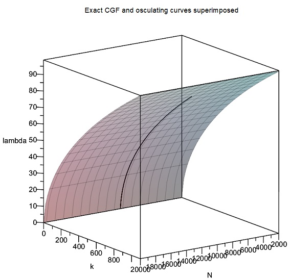
The following is a three-dimensional MAPLE plot of the cumulant generating function $\lambda(N, k;\gamma)$ for $N=0, \ldots, 10^4$ , $k=0, \ldots, 10^4$ , and $\gamma=2$ :

A simple idea from differential geometry

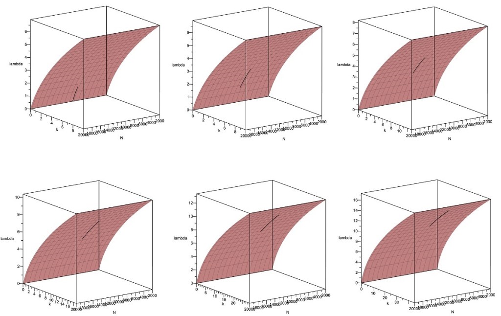
It is known in classical differential geometry that a smooth and strictly concave curve has an osculating parabola at each of its points. (See, e.g., Har’el, Z., 1995, Curvature of Curves and Surfaces – A Parabolic Approach, URL: http://harel.org.il/zvi/docs/parabola.pdf, and references therein). In particular, the curve at each point should match a Taylor expansion of the function around that point at least up to second-order. Some experiments in MAPLE indicated that remarkably accurate fits to the strictly concave $k$ -curves of the cumulant generating function can indeed be obtained using second-order Taylor expansions with respect to $k$ , for given values of $N$ and $\gamma$ . For example, the following are some 3D MAPLE plots showing closely fitting quadratic Taylor polynomials to different parts of the $k$ -curve for $N=10^4$ and $\gamma=2$ :

In these plots, the osculating quadratic Taylor expansions of $\lambda(N, k;\gamma)$ with respect to $k$ are shown centered at different points along the $k$ -curve. When just fifteen such quadratic pieces are spliced together, they form a quadratic spline providing an essentially perfect approximation of the cumulant generating function from $k = 0$ to $k = 1000$ , as shown below:

This suggests that numerical approximation schemes involving spline functions might be highly effective for the cumulant generating function in MW2016, and this indeed proved to be the case as discussed below.

Within each of the parabolic segments in the above plots, the cumulant generating function behaves to a very close approximation like a simple quadratic in $k$ . In fact, this applies at every point of the cumulant generating function, i.e., for every relevant value of $N$ and $k$ , and indeed for every relevant value of $\gamma$ . Before embarking on the development of spline function approximation techniques, it therefore seems desirable to try to understand better how the large deviation theory in MW2016 manifests itself in this simple quadratic setup. To this end, suppose that $N$ and $\gamma$ are given, and consider a point $k_0$ on the corresponding $k$ -curve of the cumulant generating function. There will be a parabolic segment around this point within which the cumulant generating function behaves exactly like the following quadratic in $k$ :

$\lambda(N, k; \gamma) = \lambda(N, k_0; \gamma) + \frac{\partial \lambda(N, k_0; \gamma)}{\partial k} (k - k_0) + \frac{1}{2}\frac{\partial^2 \lambda(N, k_0; \gamma)}{\partial k^2} (k - k_0)^2 \qquad \qquad \qquad \qquad \qquad (11)$

The coefficients here are just (1), (2) and (3) above, evaluated at the given values of $N$ and $\gamma$ , and at $k_0$ . To simplify notation in what follows, we will write the partial derivatives in (11) as

$A \equiv \frac{\partial \lambda(N, k_0; \gamma)}{\partial k} = \sum_{n=1}^N \frac{1}{n^{\gamma} + k_0} \qquad \qquad \qquad \qquad \qquad (12)$

and

$B \equiv - \frac{\partial^2 \lambda(N, k_0; \gamma)}{\partial k^2} = \sum_{n=1}^N \frac{1}{(n^{\gamma} + k_0)^2} \qquad \qquad \qquad \qquad \qquad (13)$

The entropy function in MW2016 is

$J(\bar{T}) = \sup_k \{\lambda(N, k; \gamma) - k \bar{T} \} \qquad \qquad \qquad \qquad \qquad (14)$

Differentiating the expression in curly brackets with respect to $k$ and setting equal to zero in order to find $k^{\ast}(\bar{T})$ , using (11) above, we obtain

$k^{\ast}(\bar{T}) = k_0 + \frac{A - \bar{T}}{B} \qquad \qquad \qquad \qquad \qquad (15)$

This expression is interesting for two reasons. First, recall that for any given $\bar{T}$ there is a unique $k^{\ast}(\bar{T})$ . Suppose we are in fact within the parabolic segment containing $k^{\ast}(\bar{T})$ for such a given value of $\bar{T}$ . If the centre of the Taylor expansion $k_0$ for that particular parabolic segment is slightly away from $k^{\ast}(\bar{T})$ , then the required correction for the given $\bar{T}$ is represented by the second term in (15) above, which involves $A - \bar{T}$ . There is no correction needed if $k_0 = k^{\ast}(\bar{T})$ , and this happens when $\bar{T} = A$ in (15) above. But this is exactly the saddlepoint condition in equation [16] in MW2016, so one of the key equations in the large deviation theory in MW2016 has now appeared naturally in this simple quadratic setup.

The second reason that (15) seems interesting is that it resembles the well known Newton-Raphson formula used for solving equations iteratively. This suggests that (15) might actually provide an efficient way of solving $A - \bar{T}=0$ in order to find exact values of $k^{\ast}(\bar{T})$ for different values of $\bar{T}$ . Experiments in MAPLE do indeed confirm that (15) is a useful formula for quickly obtaining values of $k^{\ast}(\bar{T})$ , particularly in the case $\gamma=4/3$ with large values of $N$ , say $N=10^4$ . Using the Maximize command in MAPLE’s Optimization package, with the right-hand side of (15) as the objective function and given values of $\bar{T}$ one very quickly obtains values of $k^{\ast}(\bar{T})$ as the maximised values of the objective function. This approach is much faster in the case $\gamma=4/3$ than using MAPLE’s fsolve command directly with formula [16] in MW2016, though fsolve does work well in the case $\gamma=2$ .

Putting (15) into (11) and simplifying we get

$\lambda(N, k^{\ast}(\bar{T});\gamma) = \lambda(N, k_0; \gamma) + \frac{A^2 - \bar{T}^2}{2B} \qquad \qquad \qquad \qquad \qquad (16)$

Again, we can regard the second term here as the correction needed when the centre of the Taylor expansion $k_0$ is not quite equal to the optimal value $k^{\ast}(\bar{T})$ . Putting (16) into (14), we get the entropy function as

$J(\bar{T}) = \lambda(N, k_0; \gamma) - k_0 \bar{T} + \frac{A^2 - \bar{T}^2}{2B} \qquad \qquad \qquad \qquad \qquad (17)$

where again the last term is a correction, and, finally, the saddlepoint density in [17] in MW2016 is obtained here as

$P(\bar{T}) = \frac{1}{\sqrt{2 \pi B}} \exp(-J(\bar{T})) \qquad \qquad \qquad \qquad \qquad (18)$

This analysis indicates how the large deviation theory in MW2016 can be linked to a simple quadratic spline approximation of the cumulant generating function. The question now is how to implement these ideas computationally to obtain a spline function approximation approach which can be used to obtain rapid and accurate quantitative results for any desired values of $N$ , $k$ , $\bar{T}$ and $\gamma$ . A simple scheme immediately suggests itself, as described in the next section.

A spline approximation approach for MAPLE

The following spline function approximation approach for MAPLE implements the insights from the previous sections, and proves to work extremely well in the sense that it produces highly accurate results, very quickly, using only the simplest polynomials, and for any desired values of $N$ , $k$ , $\bar{T}$ and $\gamma$ :

a). First, we obtain a small sample of exact values of $k^{\ast}(\bar{T})$ corresponding to some given values of $\bar{T}$ between 0.01 and 2.00, using equation [16] in MW2016 or equation (15) above. Experiments show that 40 sample values are ample for highly accurate spline approximations. These sample values can be obtained very quickly using MAPLE’s fsolve or Maximize commands, as indicated in the previous section.

b). Second, we use this small sample of exact values to create spline function representations of $k^{\ast}(\bar{T})$ and $\lambda(N, k^{\ast}(\bar{T});\gamma)$ , analogous to the quadratic spline created manually for the cumulant generating function in the previous section. This quadratic spline worked very well due to the smoothness and well-behaved nature of the cumulant generating function, but even more accurate results can be obtained with cubic splines. MAPLE routines can be written which can generate such cubic spline approximations very quickly.

c). Next, we obtain the first and second derivatives of the spline function representation of $\lambda(N, k^{\ast}(\bar{T});\gamma)$ . The component pieces of this spline will all be simple cubics, so this differentiation exercise is handled very quickly by MAPLE.

d). Finally, using the cubic spline function representation of $k^{\ast}(\bar{T})$ , we can now generate fine-grained numerical data by evaluating $k^{\ast}(\bar{T})$ for as many values of $\bar{T}$ as desired, and we can also obtain the corresponding values of the spline representation of $\lambda(N, k^{\ast}(\bar{T});\gamma)$ and its derivatives. These can then be used to compute sets of fine-grained numerical values for the entropy function $J(k^{\ast}(\bar{T}))$ and the log-saddlepoint-density function $\ln(P(\bar{T}))$ . (The term fine-grained is used here to mean approximately 200 values of the relevant functions, or more, corresponding to values of $\bar{T}$ in the range 0.0 to 2.0). Note that an immediate check of accuracy can be performed at this stage by comparing the values of the first derivative of the spline $\lambda(N, k^{\ast}(\bar{T});\gamma)$ , evaluated at the fine-grained values of the spline $k^{\ast}(\bar{T})$ , with the corresponding values of $\bar{T}$ . They should closely agree if the splines are accurately interpolating the corresponding exact function values.

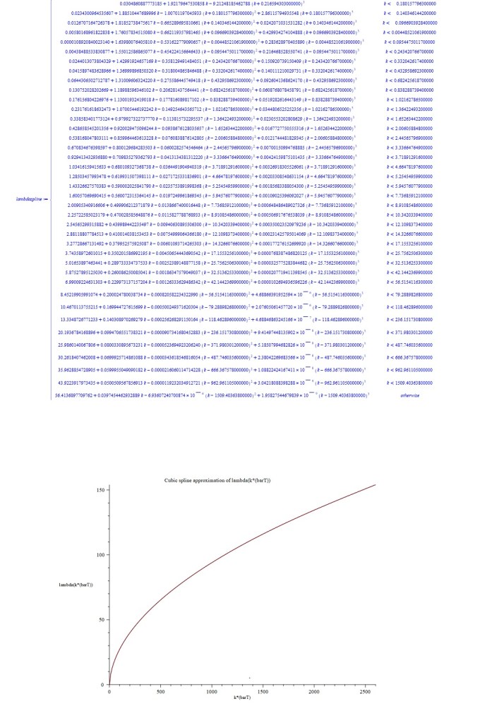
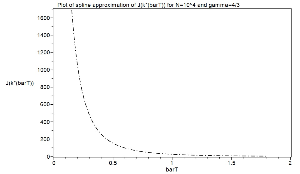
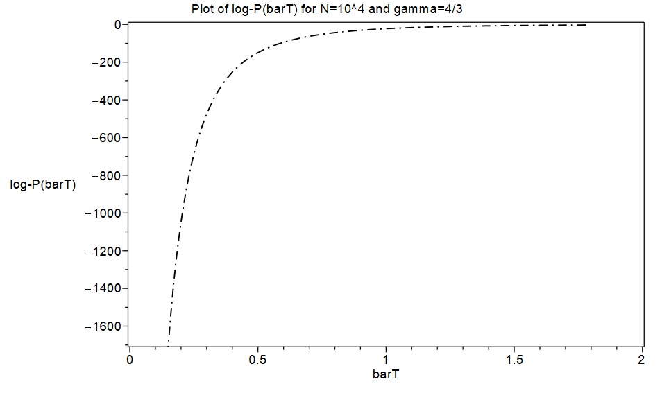
As a first excursion with this new approximation approach, an attempt was made to replicate the results in MW2016 for the cases $\gamma=2$ and $\gamma=4/3$ , with $N=10^4$ . Spline function representations of $k^{\ast}(T)$ and $\lambda(N, k^{\ast}(\bar{T});\gamma)$ consisting of 40 cubic pieces were quickly obtained with initial samples of 40 exact values of $k^{\ast}(\bar{T})$ . These are displayed below as piecewise functions for the case $\gamma=2$ , together with plots of the corresponding splines. The derivatives of $\lambda(N, k^{\ast}(\bar{T});\gamma)$ were then calculated, and these were used to calculate the entropy functions and the log-saddlepoint-density functions, finally obtaining plots of these which are also shown below for the cases $\gamma=2$ and $\gamma=4/3$ .

Note that, despite the computational difficulties encountered when trying to compute exact function values for the case $\gamma=4/3$ in particular, obtaining the corresponding cubic spline function approximations proved to be just as quick and easy as for the case $\gamma=2$ .

Checking accuracy of splines and asymptotic formulae

In the previous section, a solution system was developed based on spline function approximations that can quickly and accurately solve the large deviation problems we are interested in, for any values of $N$ , $k$ , $\bar{T}$ and $\gamma$ , even when these solutions are computationally difficult or impossible to obtain in a fine-grained way using exact functions. This gives us a machine for quickly generating accurate benchmark solutions which, for example, can be compared with analytical work.

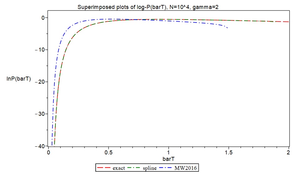
I decided to try to put both the spline function approach and the asymptotic formulae in MW2016 to the test by producing fine-grained exact values for the relevant functions (i.e., approximately 200 function values for values of $\bar{T}$ in the range 0.0 to 2.0), and then comparing our approximations with these. I was able to obtain fine-grained exact values for the case $N=10^4$ and $\gamma=2$ in MAPLE, and this took a significant amount of computation time using the relevant exact functions. In contrast, it only took a few minutes to produce corresponding spline function approximations to an equally fine-grained degree, i.e. approximately 200 values, with a discretization based on 40 values of $\bar{T}$ , giving a sample of 40 exact values of $k^{\ast}(\bar{T})$ . I also used formulas [19] and [21] in the Supplement to MW2016 to generate corresponding data based on MW’s asymptotic formulae. I then produced superimposed plots of the exact data, the spline function approximations, and the asymptotic formulae in MW2016 to visually assess accuracy.

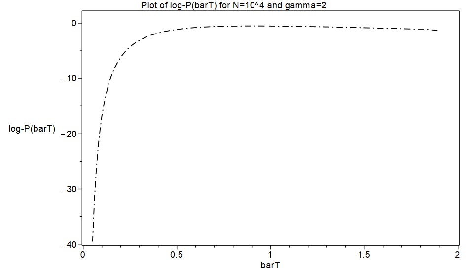
As shown in the following plots, the spline function approximations produced results in a few minutes which are essentially indistinguishable from the exact values obtained after numerous hours of computation in MAPLE. However, the asymptotic formulae in MW2016 (plots shown in blue) produced rather inaccurate approximations for $N=10^4$ and $\gamma=2$ .

In the case $\gamma=4/3$ , obtaining fine-grained exact data is computationally very time consuming in MAPLE. Exact formula computations take a lot longer with $\gamma=4/3$ than with $\gamma=2$ , and producing a fine-grained set of around 200 exact values for all the required functions with $N=10^4$ and $\gamma=4/3$ takes a large amount of computing time. However, the spline approximation approach produced such fine-grained results again in only a few minutes. In lieu of fine-grained exact function values, I used MAPLE to generate six exact function values for the case $N=10^4$ and $\gamma=4/3$ , and I plotted these as discrete points together with the spline functions to provide some degree of comparison with exact data. The results again indicate that the spline approximations are highly accurate representations of what fine-grained exact results would have looked like.

I also decided to compare the asymptotic formulae in MW2016 with the spline approximations and exact function values. I used formulae [19] and [24] in the Supplement to MW2016 for this. (MW asserts there that formula [24] produces more accurate asymptotic approximations than formula [21] in the case $\gamma=4/3$ ). In the following plots, the spline function approximations are shown in green and MW’s asymptotic formulae in blue. The six exact function values are plotted as discrete red points. As in the case $\gamma=2$ , the spline functions seem to be accurately representing the exact results, while the asymptotic formulae in MW2016 are clearly producing inaccurate results here. The discrepancies between the asymptotic formulae and the spline approximations/exact values seem a lot worse for $\gamma=4/3$ than for $\gamma=2$ , with $N=10^4$ .

On the basis of these accuracy checks, there is therefore little question that the asymptotic formulae in MW2016 are producing rather inaccurate results in the case $N=10^4$ for both $\gamma=2$ and $\gamma = 4/3$ when compared with both exact function values and my spline approximations, notwithstanding the favourable-looking numerical simulation results reported in MW2016 for log-densities. (I have communicated these results to Michael Wilkinson, the author of MW2016).

A spline approximation scheme for large deviation theory problems

Published by Dr Christian P. H. Salas

Leave a comment Cancel reply