Derivation and manipulation of a generalised Erlang distribution

The present note uses the setup outlined in a previous note about a 2016 paper in Physical Review Letters on the large deviation analysis of rapid-onset rain showers. This paper will be referred to as MW2016 herein. In order to apply large deviation theory to a collector-drop framework for rapid-onset rain formation, equation [14] in MW2016 presents the cumulant generating function for the random variable $T$ , which I will write here as

$\lambda(k) = \sum_{n=1}^{\mathcal{N}} \ln \bigg(\frac{R_n + k}{R_n}\bigg)$

The Laplace transform of the required probability density is $\exp(-\lambda(k))$ , so equation [15] in MW2016 sets up a relevant Bromwich integral equation, which I will write here as

$f_T(\bar{T}) = \frac{1}{2 \pi i} \int_{\mathcal{R}-i \infty}^{\mathcal{R}+i \infty} dz \exp(z \bar{T}) \exp(-\lambda(z)) \qquad \qquad \qquad \qquad \qquad (1)$

At first sight, this seems intractable directly, and a saddle-point approximation for the density in (1) is presented in equation [17] in MW2016. This saddle-point approximation involves the large deviation entropy function for the random variable $T$ , and an intricate asymptotic analysis is then embarked upon to obtain an explicit expression for this entropy function. The result is the expression given in equation [24] in MW2016.

However, instead of approximating (1), it is possible to work out the Bromwich integral exactly. The result is the exact version of the probability density which is approximated in equation [17] in MW2016. This is a known distribution called the generalised Erlang distribution, but I have not been able to find any derivations of it using the Bromwich integral approach. Typically, derivations are carried out using characteristic functions (see, e.g., Bibinger, M., 2013, Notes on the sum and maximum of independent exponentially distributed random variables with different scale parameters, arXiv:1307.3945 [math.PR]), or phase-type distribution methods (see, e.g., O’Cinneide, C., 1999, Phase-type distribution: open problems and a few properties, Communication in Statistic-Stochastic Models, 15(4), pp. 731-757).

To derive this distribution directly from the Bromwich integral in (1), begin by replacing the $\exp(-\lambda(k))$ term by the product it gives rise to:

$f_T(\bar{T}) = \frac{1}{2 \pi i} \int_{\mathcal{R}-i \infty}^{\mathcal{R}+i \infty} dz \exp(z \bar{T}) \prod_{n=1}^{\mathcal{N}} \bigg(\frac{R_n}{R_n+z}\bigg) \qquad \qquad \qquad \qquad \qquad (2)$

Then, starting from an elementary bivariate partial fraction expansion, and extending this to $\mathcal{N}$ variables by induction, we can obtain the following expression for the product term in (2):

$\prod_{n=1}^{\mathcal{N}} \bigg(\frac{R_n}{R_n+z}\bigg) = \sum_{n=1}^{\mathcal{N}} \bigg(\prod_{\substack{j=1 \\ j\neq n}}^{\mathcal{N}} \bigg(\frac{R_j}{R_j - R_n}\bigg)R_n \bigg(\frac{1}{R_n+z}\bigg)\bigg) \qquad \qquad \qquad \qquad \qquad (3)$

The detailed derivation of (3) is set out in an Appendix below. Putting (3) back into (2), and moving the integral sign `through’ the summation and product in (3), we obtain the following form for the Bromwich integral:

$f_T(\bar{T}) = \sum_{n=1}^{\mathcal{N}} \bigg(\prod_{\substack{j=1 \\ j\neq n}}^{\mathcal{N}} \bigg(\frac{R_j}{R_j - R_n}\bigg)R_n\bigg \{\frac{1}{2 \pi i} \int_{\mathcal{R}-i \infty}^{\mathcal{R}+i \infty} dz \frac{\exp(z \bar{T})}{R_n + z} \bigg \} \bigg) \qquad \qquad \qquad \qquad \qquad (4)$

Each integrand in (4) has a simple pole at $z = -R_n$ , so the residue at each such singularity is given by

$\lim_{z \rightarrow -R_n} \bigg((R_n + z) \frac{\exp(z \bar{T})}{(R_n + z)}\bigg) = \exp(-R_n \bar{T}) \qquad \qquad \qquad \qquad \qquad (5)$

We can construct a contour in the complex plane which is appropriate for each $R_n$ by creating a semicircle with the straight vertical part located at a point $\mathcal{R}$ to the right of $-R_1$ , and with the arc of the semicircle large enough to enclose the point $-R_{\mathcal{N}}$ on the real axis (diagram below). Since $R_1$ is the smallest collision rate, and $R_{\mathcal{N}}$ is the largest, this ensures that the contour will enclose each $-R_n$ point.

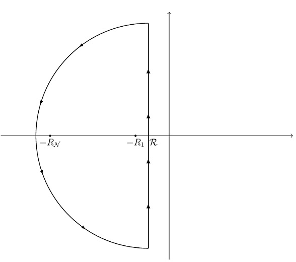
It then follows by Cauchy’s residue theorem, and the fact that the integral along the circular arc component of the contour vanishes as the radius of the semicircle goes to infinity, that

$\frac{1}{2 \pi i} \int_{\mathcal{R}-i \infty}^{\mathcal{R}+i \infty} dz \frac{\exp(z \bar{T})}{R_n + z} = \frac{1}{2 \pi i} \big (2 \pi i \exp(-R_n \bar{T}) \big) = \exp(-R_n \bar{T}) \qquad \qquad \qquad \qquad \qquad (6)$

Putting (6) in (4), we then get the exact form of the required density:

$f_T(\bar{T}) = \sum_{n=1}^{\mathcal{N}} \bigg(\prod_{\substack{j=1 \\ j\neq n}}^{\mathcal{N}} \bigg(\frac{R_j}{R_j - R_n}\bigg)R_n \exp(-R_n \bar{T}) \bigg) \qquad \qquad \qquad \qquad \qquad (7)$

This is the density function of the generalised Erlang distribution, and is given in an alternative (but equivalent) form in equation [SB1.1] on page 241 of a paper by Kostinski and Shaw (Kostinski, A., Shaw, R., 2005, Fluctuations and Luck in Droplet Growth by Coalescence, Bull. Am. Meteorol. Soc. 86, 235). Integrating (7) with respect to $\bar{T}$ , we obtain the cumulative distribution function

$F_T(\bar{T}) = \sum_{n=1}^{\mathcal{N}} \bigg(\prod_{\substack{j=1 \\ j\neq n}}^{\mathcal{N}} \bigg(\frac{R_j}{R_j - R_n}\bigg)\big (1 - \exp(-R_n \bar{T}) \big) \bigg) \qquad \qquad \qquad \qquad \qquad (8)$

Again this is given in an alternative (but equivalent) form on page 241 of Kostinski and Shaw’s paper, as equation [SB1.2].

Although we now have the exact pdf and cdf corresponding to the Bromwich integral in MW2016, these are not practical for calculations in the context of runaway raindrop growth. This runaway process can involve large numbers of water particle collisions $\mathcal{N}$ , e.g., $\mathcal{N}=10,000$ , so the expressions in (7) and (8) would involve sums of thousands of product terms, each of these products in turn involving thousands of terms. Therefore, we are still interested in obtaining a formula for the entropy function $J(\bar{T})$ to enable large deviation approximations for (7) and (8) for practical calculations. It may be possible to obtain an approximation for the entropy function directly from the cdf in (8), but this would require further investigation.

An initial problem that might need to be overcome is that the forms for the cdf in (8) above and also in Kostinski and Shaw (which is similar) are inconvenient. However, they can be manipulated as follows. First, expand (8) to obtain

$F_T(\bar{T}) = \sum_{n=1}^{\mathcal{N}} \bigg(\prod_{\substack{j=1 \\ j\neq n}}^{\mathcal{N}} \bigg(\frac{R_j}{R_j - R_n}\bigg) \bigg) - \sum_{n=1}^{\mathcal{N}} \bigg(\prod_{\substack{j=1 \\ j\neq n}}^{\mathcal{N}} \bigg(\frac{R_j}{R_j - R_n}\bigg) \exp(-R_n \bar{T})\bigg) \qquad \qquad \qquad \qquad \qquad (9)$

A recent paper by Yanev (Yanev, G., 2020, Exponential and Hypoexponential Distributions: Some Characterizations, Mathematics, 8(12), 2207) pointed out that the product terms appearing in (9) are related to the terms appearing in the Lagrange polynomial interpolation formula. This formula and its properties are well known in the field of approximation theory (see, e.g., pages 33-35 in Powell, M., 1981, Approximation Theory and Methods, Cambridge University Press). This fact was used in a paper by Sen and Balakrishnan (Sen, A., Balakrishnan, N., 1999, Convolution of geometrics and a reliability problem, Statistics & Probability Letters, 43, pp. 421-426) to give a simple proof that the sum/product which appears as the first term on the right-hand side of (9) is identically equal to 1:

$\sum_{n=1}^{\mathcal{N}} \bigg(\prod_{\substack{j=1 \\ j\neq n}}^{\mathcal{N}} \bigg(\frac{R_j}{R_j - R_n}\bigg) \bigg) \equiv 1 \qquad \qquad \qquad \qquad \qquad (10)$

(See my previous note about this). Using (10) in (9), we then obtain the cdf in a potentially more convenient form:

$F_T(\bar{T}) = 1 - \sum_{n=1}^{\mathcal{N}} \bigg(\prod_{\substack{j=1 \\ j\neq n}}^{\mathcal{N}} \bigg(\frac{R_j}{R_j - R_n}\bigg) \exp(-R_n \bar{T})\bigg) \qquad \qquad \qquad \qquad \qquad (11)$

Appendix: Proof of the partial fraction expansion in (3)

The following arguments use the Lagrange polynomial interpolation formula to prove the partial fraction expansion in (3) above. We will need formula (6) in my previous note about this, which is repeated here for convenience:

$p(R) = \sum_{n=1}^{\mathcal{N}} \bigg(\prod_{\substack{j=1 \\ j\neq n}}^{\mathcal{N}} \bigg(\frac{R_j - R}{R_j - R_n}\bigg) \bigg) \cdot 1 \qquad \qquad \qquad (12)$

To prove (3) above, we begin by using Lagrange’s polynomial interpolation formula to prove the following auxiliary result:

$\sum_{n=1}^{\mathcal{N}} \prod_{\substack{j=1 \\ j\neq n}}^{\mathcal{N}} \bigg(\frac{R_j}{R_j - R_n}\bigg)\bigg(\frac{R_n}{R_n - R_{\mathcal{N}+1}}\bigg) = \prod_{j=1}^{\mathcal{N}} \bigg(\frac{R_j}{R_j - R_{\mathcal{N}+1}}\bigg) \qquad \qquad \qquad (13)$

Taking apart (12) above (which equals 1) and using (10) above, we obtain

$\sum_{n=1}^{\mathcal{N}} \bigg(\prod_{\substack{j=1 \\ j\neq n}}^{\mathcal{N}} \bigg(\frac{R_j - R}{R_j - R_n}\bigg) \bigg)$

$= \sum_{n=1}^{\mathcal{N}} \bigg(\prod_{\substack{j=1 \\ j\neq n}}^{\mathcal{N}} \bigg(\frac{R_j}{R_j - R_n}\bigg) \bigg) - \sum_{n=1}^{\mathcal{N}} \bigg(\prod_{\substack{j=1 \\ j\neq n}}^{\mathcal{N}} \bigg(\frac{R}{R_j - R_n}\bigg) \bigg)$

$= 1 - R \sum_{n=1}^{\mathcal{N}} \bigg(\prod_{\substack{j=1 \\ j\neq n}}^{\mathcal{N}} \bigg(\frac{1}{R_j - R_n}\bigg) \bigg) = 1 \qquad \qquad \qquad (14)$

Therefore we conclude

$\sum_{n=1}^{\mathcal{N}} \bigg(\prod_{\substack{j=1 \\ j\neq n}}^{\mathcal{N}} \bigg(\frac{1}{R_j - R_n}\bigg) \bigg) = 0 \qquad \qquad \qquad (15)$

We will need this result shortly. Next, we expand the bracketed terms on the left-hand side of (13) by partial fractions. We write

$\frac{R_j R_n}{(R_j - R_n)(R_n - R_{\mathcal{N}+1})} = \frac{AR_j R_n}{(R_j - R_n)} + \frac{B R_j R_n}{(R_n - R_{\mathcal{N}+1})} \qquad \qquad \qquad (16)$

where $A$ and $B$ are to be determined. Therefore

$1 = (A - B) R_n - A R_{\mathcal{N}+1} + B R_j \qquad \qquad \qquad (17)$

Upon setting $A = B$ , (17) yields

$A = B = \frac{1}{(R_j - R_{\mathcal{N}+1})} \qquad \qquad \qquad (18)$

Putting (18) in (16), we see that the left-hand side of (13) becomes

$\sum_{n=1}^{\mathcal{N}} \prod_{\substack{j=1 \\ j\neq n}}^{\mathcal{N}} \bigg \{\bigg(\frac{R_j}{R_j - R_{\mathcal{N}+1}}\bigg)\bigg(\frac{R_n}{R_n - R_{\mathcal{N}+1}}\bigg) + \bigg(\frac{R_j}{R_j - R_{\mathcal{N}+1}}\bigg)\bigg(\frac{R_n}{R_j - R_n}\bigg)\bigg \}$

$= \sum_{n=1}^{\mathcal{N}} \prod_{\substack{j=1 \\ j\neq n}}^{\mathcal{N}} \bigg(\frac{R_j}{R_j - R_{\mathcal{N}+1}}\bigg) \bigg \{ \bigg(\frac{R_n}{R_n - R_{\mathcal{N}+1}}\bigg) - \bigg(\frac{R_n}{R_n - R_j}\bigg)\bigg \} \qquad \qquad \qquad (19)$

Now, the term in curly brackets in (19) is

$\frac{R_n}{R_n - R_{\mathcal{N}+1}} - \frac{R_n}{R_n - R_j} = \frac{R_n(R_{\mathcal{N}+1} - R_j)}{(R_n - R_{\mathcal{N}+1})(R_j - R_n)}$

$= \bigg(\frac{R_n}{R_n - R_{\mathcal{N}+1}}\bigg)\bigg(\frac{R_{\mathcal{N}+1}}{R_n - R_j}\bigg) + \bigg(\frac{R_n}{R_n - R_{\mathcal{N}+1}}\bigg)\bigg(\frac{R_j}{R_j - R_n}\bigg) \qquad \qquad \qquad (20)$

Therefore (19) becomes

$\sum_{n=1}^{\mathcal{N}} \prod_{\substack{j=1 \\ j\neq n}}^{\mathcal{N}} \bigg(\frac{R_j}{R_j - R_{\mathcal{N}+1}}\bigg)\bigg(\frac{R_n}{R_n - R_{\mathcal{N}+1}}\bigg)\bigg(\frac{R_{\mathcal{N}+1}}{R_n - R_j}\bigg)$

$+ \sum_{n=1}^{\mathcal{N}} \prod_{\substack{j=1 \\ j\neq n}}^{\mathcal{N}} \bigg(\frac{R_j}{R_j - R_{\mathcal{N}+1}}\bigg)\bigg(\frac{R_n}{R_n - R_{\mathcal{N}+1}}\bigg)\bigg(\frac{R_j}{R_j - R_n}\bigg)$

$= R_{\mathcal{N}+1}\prod_{j=1}^{\mathcal{N}} \bigg(\frac{R_j}{R_j - R_{\mathcal{N}+1}}\bigg) \bigg[\sum_{n=1}^{\mathcal{N}} \prod_{\substack{j=1 \\ j\neq n}}^{\mathcal{N}} \bigg(\frac{1}{R_n - R_j}\bigg) \bigg]$

$+ \prod_{j=1}^{\mathcal{N}} \bigg(\frac{R_j}{R_j - R_{\mathcal{N}+1}}\bigg) \bigg[\sum_{n=1}^{\mathcal{N}} \prod_{\substack{j=1 \\ j\neq n}}^{\mathcal{N}} \bigg(\frac{R_j}{R_j - R_n}\bigg) \bigg]$

$= \prod_{j=1}^{\mathcal{N}} \bigg(\frac{R_j}{R_j - R_{\mathcal{N}+1}}\bigg) \qquad \qquad \qquad (21)$

The last equality follows because the first term in the penultimate step is zero by (15) above, and the sum in the square brackets in the second term in the penultimate step is equal to 1 by (10) above. Therefore the auxiliary result in (13) is now proved.

Now we use this result to prove (3) by mathematical induction. As the basis for the induction, we can use the case $\mathcal{N} = 3$ which is easy to prove by repeated bivariate partial fraction expansions, and clearly exhibits the pattern represented by (3):

$\prod_{n=1}^{3} \bigg(\frac{R_n}{R_n+z}\bigg)$

$= \bigg(\frac{R_1}{R_1 + z}\bigg)\bigg(\frac{R_2}{R_2 + z}\bigg)\bigg(\frac{R_3}{R_3 + z}\bigg)$

$= \bigg(\frac{R_2}{R_2 - R_1}\bigg)\bigg(\frac{R_3}{R_3 - R_1}\bigg)\bigg(\frac{R_1}{R_1 + z}\bigg)$

$+ \bigg(\frac{R_1}{R_1 - R_2}\bigg)\bigg(\frac{R_3}{R_3 - R_2}\bigg)\bigg(\frac{R_2}{R_2 + z}\bigg)$

$+ \bigg(\frac{R_1}{R_1 - R_3}\bigg)\bigg(\frac{R_2}{R_2 - R_3}\bigg)\bigg(\frac{R_3}{R_3 + z}\bigg)$

$= \sum_{n=1}^{3} \bigg(\prod_{\substack{j=1 \\ j\neq n}}^{3} \bigg(\frac{R_j}{R_j - R_n}\bigg)R_n \bigg(\frac{1}{R_n+z}\bigg)\bigg)$

Next, suppose (3) is true. Then adding another factor to the product on the left-hand side of (3) would produce

$\prod_{n=1}^{\mathcal{N}+1} \bigg(\frac{R_n}{R_n+z}\bigg) = \sum_{n=1}^{\mathcal{N}} \bigg(\prod_{\substack{j=1 \\ j\neq n}}^{\mathcal{N}} \bigg(\frac{R_j}{R_j - R_n}\bigg)R_n \bigg) \bigg(\frac{R_{\mathcal{N}+1}}{(R_n+z)(R_{\mathcal{N}+1}+z)}\bigg)$

$= \sum_{n=1}^{\mathcal{N}} \bigg(\prod_{\substack{j=1 \\ j\neq n}}^{\mathcal{N}} \bigg(\frac{R_j}{R_j - R_n}\bigg)R_n \bigg) \bigg \{\bigg(\frac{R_{\mathcal{N}+1}}{R_{\mathcal{N}+1}-R_n}\bigg)\bigg(\frac{1}{R_n+z}\bigg)+\bigg(\frac{1}{R_n-R_{\mathcal{N}+1}}\bigg)\bigg(\frac{R_{\mathcal{N}+1}}{R_{\mathcal{N}+1}+z}\bigg)\bigg \}$

$= \sum_{n=1}^{\mathcal{N}} \prod_{\substack{j=1 \\ j\neq n}}^{\mathcal{N}} \bigg(\frac{R_j}{R_j - R_n}\bigg)\bigg(\frac{R_{\mathcal{N}+1}}{R_{\mathcal{N}+1}-R_n}\bigg)\bigg(\frac{R_n}{R_n+z}\bigg)$

$+ \bigg[\sum_{n=1}^{\mathcal{N}} \prod_{\substack{j=1 \\ j\neq n}}^{\mathcal{N}} \bigg(\frac{R_j}{R_j - R_n}\bigg)\bigg(\frac{R_n}{R_n - R_{\mathcal{N}+1}}\bigg)R_{\mathcal{N}+1}\bigg]\bigg(\frac{1}{R_{\mathcal{N}+1}+z}\bigg)$

$= \sum_{n=1}^{\mathcal{N}} \prod_{\substack{j=1 \\ j\neq n}}^{\mathcal{N}+1} \bigg(\frac{R_j}{R_j - R_n}\bigg)R_n\bigg(\frac{1}{R_n+z}\bigg)$

$+ \bigg[\prod_{j=1}^{\mathcal{N}} \bigg(\frac{R_j}{R_j - R_{\mathcal{N}+1}}\bigg)R_{\mathcal{N}+1}\bigg]\bigg(\frac{1}{R_{\mathcal{N}+1}+z}\bigg)$

$= \sum_{n=1}^{\mathcal{N}+1} \bigg(\prod_{\substack{j=1 \\ j\neq n}}^{\mathcal{N}+1} \bigg(\frac{R_j}{R_j - R_n}\bigg)R_n \bigg(\frac{1}{R_n+z}\bigg)\bigg) \qquad \qquad \qquad (22)$

where the expressions in square brackets in the two steps before the last are equal by the auxiliary result (13) proved earlier. Therefore, by the principle of mathematical induction, (3) must hold for all $\mathcal{N} \geq 3$ , so (3) is proved.

Derivation and manipulation of a generalised Erlang distribution

Published by Dr Christian P. H. Salas

Leave a comment Cancel reply