Equivalent integral formulae for Bessel functions of the first kind, order zero

Bessel’s equation arises in countless physics applications and has the form

$x^2 y^{\prime \prime} + x y^{\prime} + (x^2 - p^2) y = 0 \qquad \qquad \qquad \qquad \qquad (1)$

where the constant $p$ is known as the order of the Bessel function $y$ which solves (1). The method of Frobenius can be used to find series solutions for $y$ of the form

$y = x^s \sum_{n=0}^{\infty} a_n x^n = \sum_{n=0}^{\infty} a_n x^{n+s} = a_0 x^s + a_1 x^{s+1} + a_2 x^{s+2} + \cdots \qquad \qquad \qquad \qquad \qquad (2)$

where $s$ is a number to be found by substituting (2) and its relevant derivatives into (1). We assume that $a_0$ is not zero, so the first term of the series will be $a_0 x^s$ . Successive differentiation of (2) and substitution into (1) produces for each power of $x$ in (2) an equation equal to zero involving combinations of several coefficients $a_n$ . (The total coefficient of each power of $x$ must be zero to ensure the right-hand side of (1) ends up as zero). The equation for the coefficient of $x^s$ is used to find the possible values of $s$ and is known as the indicial equation. For the Bessel equation in (1), this procedure results in the indicial equation

$s^2 - p^2 = 0$

so $s = \pm p$ and we need to find two solutions, one for $s=p$ and another for $s = -p$ . A linear combination of these two solutions can then be used to construct a general solution of (1). The Frobenius procedure also leads to $a_1$ = 0 and the following recursion formula for the remaining coefficients:

$a_n = -\frac{a_{n-2}}{(n+s)^2 - p^2} \qquad \qquad \qquad \qquad \qquad (3)$

We use this to find coefficients for $s = p$ first, and can then simply replace $p$ by $-p$ to get the coefficients for $s = -p$ . Here, we focus only on the case $s = p$ which upon substitution in (3) gives

$a_n = -\frac{a_{n-2}}{(n+p)^2 - p^2} = -\frac{a_{n-2}}{n(n+2p)} \qquad \qquad \qquad \qquad \qquad (4)$

Evaluating these coefficients with a starting value of $a_0 = \frac{1}{2^p p!}$ results in solutions called Bessel functions of the first kind and order $p$ , usually denoted by $J_p(x)$ . In the present note, I am concerned only with the Bessel function of the first kind and order zero, $J_0(x)$ , obtained by setting $p = 0$ . We then have a starting value $a_0 = 1$ and we obtain the following coefficients in the power series for $J_0(x)$ :

$a_0 = 1$

$a_1 = 0$

$a_2 = -\frac{a_0}{2(2+0)} = -\frac{1}{4} = -\frac{1}{2^2}$

$a_3 = 0$

$a_4 = -\frac{a_2}{4(4 + 0)} = \frac{1}{2^2 \cdot 4^2}$

$a_5 = 0$

$a_6 = -\frac{a_4}{6(6 + 0)} = -\frac{1}{2^2 \cdot 4^2 \cdot 6^2}$

and so on. So, $a_1 = 0$ leads to all odd-numbered coefficients being zero and we end up with the following generalized series expression for the Bessel function of the first kind and order zero:

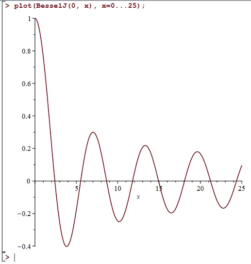
$J_0(x) = 1 - \frac{x^2}{2^2} + \frac{x^4}{2^2 \cdot 4^2} - \frac{x^6}{2^2 \cdot 4^2 \cdot 6^2} + \cdots \qquad \qquad \qquad \qquad \qquad (5)$

We can easily plot $J_0(x)$ using MAPLE and it looks like a kind of damped cosine function. Here is a quick plot for positive values of $x$ :

The series in (5) above is given, albeit in a more general complex variable setting, as equation (3) on page 16 in the classic work by G. N. Watson, 1922, A Treatise On The Theory of Bessel Functions, Cambridge University Press. (At the time of writing, this monumental book is freely downloadable from several online sites). In the present note, I am interested in certain integral formulae which give rise to the same series as (5). These are discussed in Chapter Two of Watson’s treatise, and I want to unpick some things from there. In particular, I am intrigued by the following passage on pages 19 and 20 of Watson’s book:

In the remainder of this note, I want to obtain the series for $J_0(x)$ in (5) above directly from the integral in equation (1) in this extract from Watson’s book, adapted to the real-variable case with $n = 0$ . I also want to use Watson’s technique of bisecting the range of integration to obtain a clear intuitive understanding of other equivalent integral formulae for $J_0(x)$ .

Begin by setting $n = 0$ and $z = x$ in the integral in (1) in the extract to get

$J_0(x) = \frac{1}{2 \pi }\int_0^{2 \pi} \cos(x \sin \theta) d \theta \qquad \qquad \qquad \qquad \qquad (6)$

To confirm the validity of this, we can substitute $x \sin \theta$ into the Taylor series expansion for $\cos x$ , namely

$\cos x = 1 - \frac{x^2}{2!} + \frac{x^4}{4!} - \frac{x^6}{6!} + \cdots$

to get

$\cos(x \sin \theta) = 1 - \frac{(x \sin \theta)^2}{2!} + \frac{(x \sin \theta)^4}{4!} - \frac{(x \sin \theta)^6}{6!} + \cdots \qquad \qquad \qquad \qquad \qquad (7)$

Now integrate both sides of (7) from $0$ to $2 \pi$ , using a formula I explored in a previous note for integrating even powers of the sine function, namely

$\int_0^{2 \pi} \sin^n \theta d \theta = \left\{ \begin{array}{rl} 0 & \text{for } n \text{ odd} \\ \frac{(n-1)(n-3) \cdots 3 \cdot 1}{n(n-2) \cdots 4 \cdot 2} \cdot 2 \pi & \text{for } n \text{ even} \end{array} \right. \qquad \qquad \qquad \qquad \qquad (8)$

We obtain

$\int_0^{2 \pi} \cos(x \sin \theta) d \theta = 2 \pi - \frac{x^2}{2!} \frac{1}{2} 2 \pi + \frac{x^4}{4!} \frac{3 \cdot 1}{4 \cdot 2} 2 \pi - \frac{x^6}{6!} \frac{5 \cdot 3 \cdot 1}{6 \cdot 4 \cdot 2} 2\pi + \cdots$

$= 2\pi \big(1 - \frac{x^2}{2^2} + \frac{x^4}{2^2 \cdot 4^2} - \frac{x^6}{2^2 \cdot 4^2 \cdot 6^2} + \cdots\big)$

$\frac{1}{2 \pi} \int_0^{2 \pi} \cos(x \sin \theta) d \theta = 1 - \frac{x^2}{2^2} + \frac{x^4}{2^2 \cdot 4^2} - \frac{x^6}{2^2 \cdot 4^2 \cdot 6^2} + \cdots \qquad \qquad \qquad \qquad \qquad (9)$

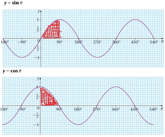
Thus, (6) holds. Notice that the integral in (6) is the average value of the integrand over the interval from $0$ to $2 \pi$ . Looking at graphs of the sine and cosine functions, we can easily imagine that we can switch between the two and that this average also remains unchanged if we restrict the range of integration to the interval from $0$ to $\frac{\pi}{2}$ , and divide the integral by $\frac{\pi}{2}$ instead of $2 \pi$ .

Thus, it seems intuitively obvious that the following are equivalent integral formulae for $J_0(x)$ :

$J_0(x) = \frac{2}{\pi} \int_0^{\pi/2} \cos(x \sin \theta) d \theta = \frac{2}{\pi} \int_0^{\pi/2} \cos(x \cos \theta) d \theta \qquad \qquad \qquad \qquad \qquad (10)$

In addition, if we substitute $i x \sin \theta$ into the Taylor series expansion for $e^x$ , namely

$e^x = 1 + \frac{x}{1!} + \frac{x^2}{2!} + \frac{x^3}{3!} + \frac{x^4}{4!} + \cdots$

we get

$e^{i x \sin \theta} = 1 + \frac{(i x \sin \theta)}{1!} + \frac{(i x \sin \theta)^2}{2!} + \frac{(i x \sin \theta)^3}{3!} + \frac{(i x \sin \theta)^4}{4!} + \cdots \qquad \qquad \qquad \qquad \qquad (11)$

But when we integrate both sides of this from $0$ to $2 \pi$ , the odd terms on the right-hand side will vanish and the even terms will be the same as they were in the derivation of (9) above using the Taylor series for cos. We thus obtain another equivalent integral formula for $J_0(x)$ :

$J_0(x) = \frac{1}{2 \pi} \int_0^{2 \pi} e^{i x \sin \theta} d \theta \qquad \qquad \qquad \qquad \qquad (12)$

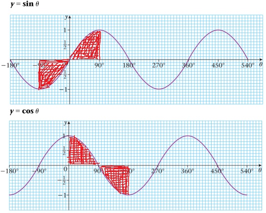
Furthermore, we can again restrict the range of integration in (12) and switch between sine and cosine as indicated in the following graphs:

Thus, we obtain the following equivalent integral formulae for $J_0(x)$ :

$J_0(x) = \frac{1}{\pi} \int_{-\pi/2}^{\pi/2} e^{i x \sin \theta} d \theta = \frac{1}{\pi} \int_0^{\pi} e^{i x \cos \theta} d \theta$

We can imagine easily obtaining many other equivalent integral formulae for $J_0(x)$ in this way.

Equivalent integral formulae for Bessel functions of the first kind, order zero

Published by Dr Christian P. H. Salas

Leave a comment Cancel reply