A mathematics and physics `scrapbook', with notes on miscellaneous things that catch my interest in a range of areas including: mathematical methods; number theory; probability theory; stochastic processes; mathematical economics; econometrics; quantum theory; relativity theory; cosmology; cloud physics; statistical mechanics; nonlinear dynamics; electronic engineering; graph and network theory; mathematics in Latin; computational mathematics using Python and other maths software.
I record here an experience of manually calculating a Fast Fourier Transform (FFT). Carrying out the computations by hand turned out to be relatively straightforward and quite instructive. A number of different FFT algorithms have been developed and the underlying equations are provided in numerous journal articles and books. I chose to calculate an eight-point (real-valued) FFT using the equations and approach discussed in the book Approximation Theory and Methods by M. J. D. Powell.
The classical Fourier analysis problem is to express a periodic function of period in the form
In the context of approximation theory, the above Fourier series is truncated so that some is the highest value of for which at least one of or is non-zero, i.e.,
We then regard as a trigonometric polynomial of degree which approximates the function (this approximation can be shown to minimise a least squares distance function).
The task is to find formulas for the coefficients and and this is achieved using the following formulas for the average values over a period of , and respectively:
Then to find the value of the coefficient in the Fourier series expansion of we take the average value of the series by integrating on term by term. We get
with all the other terms on the right-hand side equal to zero because they can all be regarded as integrals of or of with and (i.e., ). We are thus left with
This is the formula for calculating the coefficient in the Fourier series expansion of a periodic function . From then on, to find for , we multiply both sides of the generic Fourier series expansion by and again find the average value of each term to get
Analogously, to obtain the formula for , we multiply both sides of the generic Fourier series expansion by and take average values. We find
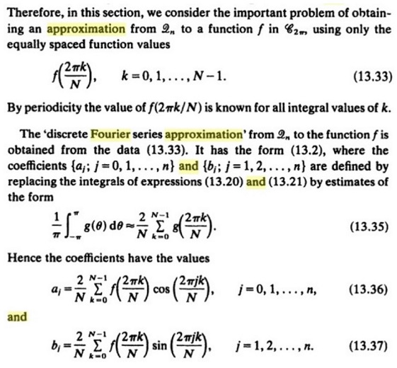
This classical setup assumes that the values of the function are known for all in the interval . When this is not the case and we only have the values of for a discrete set of points in the interval , we need to use a discretised form of Fourier series approximation. Powell approaches this in Section 13.3 of his book as follows:
Therefore the classical formulas
and
are replaced by formulas (13.36) and (13.37) in the excerpt above. To illustrate how these formulas work in a concrete example, suppose the problem is to to obtain an approximation of a function by a trigonometric polynomial of degree given only the four function values , , and . Thus, we need to obtain an approximation to of the form
Setting , we use formulas (13.36) and (13.37) to evaluate the coefficients , , , and as follows:
Therefore the required approximation is
The fast Fourier transform is designed to speed up the calculations in discrete Fourier series approximations of the above kind in cases when is large. Powell discusses this in Section 13.4 of his book as follows:
Each iteration of the FFT process depends on the value of the iteration variable , which initially is set at 1. In each subsequent iteration, the value of is set at twice the previous value, so in the second iteration we have , in the third iteration we have , in the fourth iteration we have and so on. This continues until the value of the iteration variable reaches (which in this particular FFT approach is required to be a power of ).
At the start of the first iteration we set and . Formula (13.46) then reduces to
and formula (13.47) reduces to
where for each the values of are the numbers in the set
So, in the first iteration we use the above formulas to generate values of and . We then use formulas (13.50) to obtain the numbers and . We get
Thus, the numbers and are exactly the same as the numbers and in this first iteration. At this point we are ready to begin the second iteration.
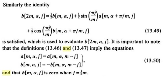
For the second iteration we double the iteration variable and use the results from the first iteration to compute the numbers and for using formulas (13.48) and (13.49). The variable runs from to in this second iteration. We then use formulas (13.50) to obtain the numbers and for and at this point we are ready to begin the third iteration.
For the third iteration we double the iteration variable again (so ) and use the results from the second iteration to compute the numbers and for using formulas (13.48) and (13.49). The variable runs from to in this third iteration. We then use formulas (13.50) to obtain the numbers and for and at this point we are ready to begin the fourth iteration.
For the fourth iteration we double the iteration variable again (so ) and use the results from the third iteration to compute the numbers and for using formulas (13.48) and (13.49). The variable runs from to in this fourth iteration. We then use formulas (13.50) to obtain the numbers and for and at this point we are ready to begin the fifth iteration.
Thus, we see that at the end of each iteration the numbers and are known, where takes all the integer values in and the variable runs from to . The iterations continue in this fashion until we arrive at the numbers and for and these provide the required coefficients for the approximation.
To illustrate how all of this works in a concrete example, I will solve a problem at the end of this chapter of Powell’s book. The problem reads as follows:
Therefore, we need to obtain an approximation to the data of the form
Applying the iterative process described above with , we begin by setting , and in formulas (13.46) and (13.47). Formula (13.46) reduces to
so we get the eight values
and formula (13.47) reduces to
which gives us
Next we calculate the numbers and using equations (13.50), which tell us that
Thus, the numbers and are exactly the same as the numbers and in this first iteration. Writing them out explicitly:
The above results can be summarised in a table for convenience:
We are now ready to begin the second iteration. The iteration variable becomes and we will have , . We compute the numbers , , and using formulas (13.48) and (13.49). We get the formulas
These then give us the values
Next we calculate the numbers and using equations (13.50), which tell us that
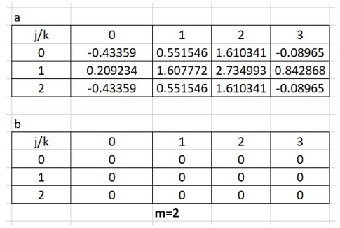
Thus, the numbers and are exactly the same as the numbers and in the second iteration. Writing them out explicitly:
The above results are summarised in the following table for convenience:
We are now ready to begin the third iteration. The iteration variable becomes and we will have , . We compute the numbers , , , , and using formulas (13.48) and (13.49). We get the formulas
These then give us the values
Next we calculate the numbers , , and using equations (13.50), which tell us that
Thus, we can use the previously computed values for and in the third iteration to get these. Writing them out explicitly:
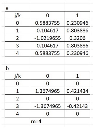
The above results are summarised in the following table:
We are now ready to begin the fourth (and final) iteration. The iteration variable becomes and we have , . We compute the numbers , , , , , , , , and using formulas (13.48) and (13.49). We get
The above results are summarised in the following table:
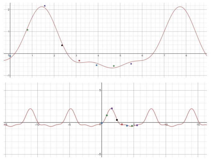
The required approximation is then
The graph of is plotted in the figures below for comparison with the initial data (the second figure shows more of the periodic pattern):


![q(x) = \frac{1}{2}a_0 + \sum_{j=1}^n\big[a_j \cos(jx) + b_j \sin(jx) \big]](https://s0.wp.com/latex.php?latex=q%28x%29+%3D+%5Cfrac%7B1%7D%7B2%7Da_0+%2B+%5Csum_%7Bj%3D1%7D%5En%5Cbig%5Ba_j+%5Ccos%28jx%29+%2B+b_j+%5Csin%28jx%29+%5Cbig%5D&bg=ffffff&fg=111111&s=0&c=20201002)


![[-\pi, \pi]](https://s0.wp.com/latex.php?latex=%5B-%5Cpi%2C+%5Cpi%5D&bg=ffffff&fg=111111&s=0&c=20201002)


![q(x) = \frac{1}{2}a_0 + \sum_{j=1}^2\big[a_j \cos(jx) + b_j \sin(jx) \big]](https://s0.wp.com/latex.php?latex=q%28x%29+%3D+%5Cfrac%7B1%7D%7B2%7Da_0+%2B+%5Csum_%7Bj%3D1%7D%5E2%5Cbig%5Ba_j+%5Ccos%28jx%29+%2B+b_j+%5Csin%28jx%29+%5Cbig%5D&bg=ffffff&fg=111111&s=0&c=20201002)


![= \frac{2}{4} \big[f(0)\cos(0) + f\big(\frac{2\pi}{4}\big) + f\big(\frac{4\pi}{4}\big) + f\big(\frac{6\pi}{4}\big)\big] = 0.975](https://s0.wp.com/latex.php?latex=%3D+%5Cfrac%7B2%7D%7B4%7D+%5Cbig%5Bf%280%29%5Ccos%280%29+%2B+f%5Cbig%28%5Cfrac%7B2%5Cpi%7D%7B4%7D%5Cbig%29+%2B+f%5Cbig%28%5Cfrac%7B4%5Cpi%7D%7B4%7D%5Cbig%29+%2B+f%5Cbig%28%5Cfrac%7B6%5Cpi%7D%7B4%7D%5Cbig%29%5Cbig%5D+%3D+0.975&bg=ffffff&fg=111111&s=0&c=20201002)
![a_1 = \frac{2}{4} \big[f(0)\cos(0) + f\big(\frac{2\pi}{4}\big)\cos\big(\frac{2\pi}{4}\big) + f\big(\frac{4\pi}{4}\big)\cos\big(\frac{4\pi}{4}\big) + f\big(\frac{6\pi}{4}\big)\cos\big(\frac{6\pi}{4}\big)\big] = -0.4](https://s0.wp.com/latex.php?latex=a_1+%3D+%5Cfrac%7B2%7D%7B4%7D+%5Cbig%5Bf%280%29%5Ccos%280%29+%2B+f%5Cbig%28%5Cfrac%7B2%5Cpi%7D%7B4%7D%5Cbig%29%5Ccos%5Cbig%28%5Cfrac%7B2%5Cpi%7D%7B4%7D%5Cbig%29+%2B+f%5Cbig%28%5Cfrac%7B4%5Cpi%7D%7B4%7D%5Cbig%29%5Ccos%5Cbig%28%5Cfrac%7B4%5Cpi%7D%7B4%7D%5Cbig%29+%2B+f%5Cbig%28%5Cfrac%7B6%5Cpi%7D%7B4%7D%5Cbig%29%5Ccos%5Cbig%28%5Cfrac%7B6%5Cpi%7D%7B4%7D%5Cbig%29%5Cbig%5D+%3D+-0.4&bg=ffffff&fg=111111&s=0&c=20201002)
![a_2 = \frac{2}{4} \big[f(0)\cos(0) + f\big(\frac{2\pi}{4}\big)\cos\big(\frac{4\pi}{4}\big) + f\big(\frac{4\pi}{4}\big)\cos\big(\frac{8\pi}{4}\big) + f\big(\frac{6\pi}{4}\big)\cos\big(\frac{12\pi}{4}\big)\big] = 0.225](https://s0.wp.com/latex.php?latex=a_2+%3D+%5Cfrac%7B2%7D%7B4%7D+%5Cbig%5Bf%280%29%5Ccos%280%29+%2B+f%5Cbig%28%5Cfrac%7B2%5Cpi%7D%7B4%7D%5Cbig%29%5Ccos%5Cbig%28%5Cfrac%7B4%5Cpi%7D%7B4%7D%5Cbig%29+%2B+f%5Cbig%28%5Cfrac%7B4%5Cpi%7D%7B4%7D%5Cbig%29%5Ccos%5Cbig%28%5Cfrac%7B8%5Cpi%7D%7B4%7D%5Cbig%29+%2B+f%5Cbig%28%5Cfrac%7B6%5Cpi%7D%7B4%7D%5Cbig%29%5Ccos%5Cbig%28%5Cfrac%7B12%5Cpi%7D%7B4%7D%5Cbig%29%5Cbig%5D+%3D+0.225&bg=ffffff&fg=111111&s=0&c=20201002)

![= \frac{2}{4} \big[f(0)\sin(0) + f\big(\frac{2\pi}{4}\big)\sin\big(\frac{2\pi}{4}\big) + f\big(\frac{4\pi}{4}\big)\sin\big(\frac{4\pi}{4}\big) + f\big(\frac{6\pi}{4}\big)\sin\big(\frac{6\pi}{4}\big)\big] = -0.125](https://s0.wp.com/latex.php?latex=%3D+%5Cfrac%7B2%7D%7B4%7D+%5Cbig%5Bf%280%29%5Csin%280%29+%2B+f%5Cbig%28%5Cfrac%7B2%5Cpi%7D%7B4%7D%5Cbig%29%5Csin%5Cbig%28%5Cfrac%7B2%5Cpi%7D%7B4%7D%5Cbig%29+%2B+f%5Cbig%28%5Cfrac%7B4%5Cpi%7D%7B4%7D%5Cbig%29%5Csin%5Cbig%28%5Cfrac%7B4%5Cpi%7D%7B4%7D%5Cbig%29+%2B+f%5Cbig%28%5Cfrac%7B6%5Cpi%7D%7B4%7D%5Cbig%29%5Csin%5Cbig%28%5Cfrac%7B6%5Cpi%7D%7B4%7D%5Cbig%29%5Cbig%5D+%3D+-0.125&bg=ffffff&fg=111111&s=0&c=20201002)
![b_2 = \frac{2}{4} \big[f(0)\sin(0) + f\big(\frac{2\pi}{4}\big)\sin\big(\frac{4\pi}{4}\big) + f\big(\frac{4\pi}{4}\big)\sin\big(\frac{8\pi}{4}\big) + f\big(\frac{6\pi}{4}\big)\sin\big(\frac{12\pi}{4}\big)\big] = 0](https://s0.wp.com/latex.php?latex=b_2+%3D+%5Cfrac%7B2%7D%7B4%7D+%5Cbig%5Bf%280%29%5Csin%280%29+%2B+f%5Cbig%28%5Cfrac%7B2%5Cpi%7D%7B4%7D%5Cbig%29%5Csin%5Cbig%28%5Cfrac%7B4%5Cpi%7D%7B4%7D%5Cbig%29+%2B+f%5Cbig%28%5Cfrac%7B4%5Cpi%7D%7B4%7D%5Cbig%29%5Csin%5Cbig%28%5Cfrac%7B8%5Cpi%7D%7B4%7D%5Cbig%29+%2B+f%5Cbig%28%5Cfrac%7B6%5Cpi%7D%7B4%7D%5Cbig%29%5Csin%5Cbig%28%5Cfrac%7B12%5Cpi%7D%7B4%7D%5Cbig%29%5Cbig%5D+%3D+0&bg=ffffff&fg=111111&s=0&c=20201002)


![a[1, \alpha, 0] = 2f(\alpha)](https://s0.wp.com/latex.php?latex=a%5B1%2C+%5Calpha%2C+0%5D+%3D+2f%28%5Calpha%29&bg=ffffff&fg=111111&s=0&c=20201002)
![b[1, \alpha, 0] = 0](https://s0.wp.com/latex.php?latex=b%5B1%2C+%5Calpha%2C+0%5D+%3D+0&bg=ffffff&fg=111111&s=0&c=20201002)


![a[1, \alpha, 0]](https://s0.wp.com/latex.php?latex=a%5B1%2C+%5Calpha%2C+0%5D&bg=ffffff&fg=111111&s=0&c=20201002)
![b[1, \alpha, 0]](https://s0.wp.com/latex.php?latex=b%5B1%2C+%5Calpha%2C+0%5D&bg=ffffff&fg=111111&s=0&c=20201002)
![a[1, \alpha, 1]](https://s0.wp.com/latex.php?latex=a%5B1%2C+%5Calpha%2C+1%5D&bg=ffffff&fg=111111&s=0&c=20201002)
![b[1, \alpha, 1]](https://s0.wp.com/latex.php?latex=b%5B1%2C+%5Calpha%2C+1%5D&bg=ffffff&fg=111111&s=0&c=20201002)
![a[1, \alpha, 1] = a[1, \alpha, 0] = 2f(\alpha)](https://s0.wp.com/latex.php?latex=a%5B1%2C+%5Calpha%2C+1%5D+%3D+a%5B1%2C+%5Calpha%2C+0%5D+%3D+2f%28%5Calpha%29&bg=ffffff&fg=111111&s=0&c=20201002)
![b[1, \alpha, 1] = -b[1, \alpha, 0] = 0](https://s0.wp.com/latex.php?latex=b%5B1%2C+%5Calpha%2C+1%5D+%3D+-b%5B1%2C+%5Calpha%2C+0%5D+%3D+0&bg=ffffff&fg=111111&s=0&c=20201002)
![a[2, \alpha, j]](https://s0.wp.com/latex.php?latex=a%5B2%2C+%5Calpha%2C+j%5D&bg=ffffff&fg=111111&s=0&c=20201002)
![b[2, \alpha, j]](https://s0.wp.com/latex.php?latex=b%5B2%2C+%5Calpha%2C+j%5D&bg=ffffff&fg=111111&s=0&c=20201002)


![a[4, \alpha, j]](https://s0.wp.com/latex.php?latex=a%5B4%2C+%5Calpha%2C+j%5D&bg=ffffff&fg=111111&s=0&c=20201002)
![b[4, \alpha, j]](https://s0.wp.com/latex.php?latex=b%5B4%2C+%5Calpha%2C+j%5D&bg=ffffff&fg=111111&s=0&c=20201002)


![a[8, \alpha, j]](https://s0.wp.com/latex.php?latex=a%5B8%2C+%5Calpha%2C+j%5D&bg=ffffff&fg=111111&s=0&c=20201002)
![b[8, \alpha, j]](https://s0.wp.com/latex.php?latex=b%5B8%2C+%5Calpha%2C+j%5D&bg=ffffff&fg=111111&s=0&c=20201002)


![a[m, \alpha, j]](https://s0.wp.com/latex.php?latex=a%5Bm%2C+%5Calpha%2C+j%5D&bg=ffffff&fg=111111&s=0&c=20201002)
![b[m, \alpha, j]](https://s0.wp.com/latex.php?latex=b%5Bm%2C+%5Calpha%2C+j%5D&bg=ffffff&fg=111111&s=0&c=20201002)
![[0, m]](https://s0.wp.com/latex.php?latex=%5B0%2C+m%5D&bg=ffffff&fg=111111&s=0&c=20201002)

![a_j = a[N, 0, j]](https://s0.wp.com/latex.php?latex=a_j+%3D+a%5BN%2C+0%2C+j%5D&bg=ffffff&fg=111111&s=0&c=20201002)
![b_j = b[N, 0, j]](https://s0.wp.com/latex.php?latex=b_j+%3D+b%5BN%2C+0%2C+j%5D&bg=ffffff&fg=111111&s=0&c=20201002)


![q(x) = \frac{1}{2}a_0 + \sum_{j=1}^3\big[a_j \cos(jx) + b_j \sin(jx) \big]](https://s0.wp.com/latex.php?latex=q%28x%29+%3D+%5Cfrac%7B1%7D%7B2%7Da_0+%2B+%5Csum_%7Bj%3D1%7D%5E3%5Cbig%5Ba_j+%5Ccos%28jx%29+%2B+b_j+%5Csin%28jx%29+%5Cbig%5D&bg=ffffff&fg=111111&s=0&c=20201002)


![a\big[1, \frac{2\pi \cdot 0}{8}, 0\big] = 2f\big(\frac{2\pi \cdot 0}{8}\big) = -0.224356](https://s0.wp.com/latex.php?latex=a%5Cbig%5B1%2C+%5Cfrac%7B2%5Cpi+%5Ccdot+0%7D%7B8%7D%2C+0%5Cbig%5D+%3D+2f%5Cbig%28%5Cfrac%7B2%5Cpi+%5Ccdot+0%7D%7B8%7D%5Cbig%29+%3D+-0.224356&bg=ffffff&fg=111111&s=0&c=20201002)
![a\big[1, \frac{2\pi \cdot 1}{8}, 0\big] = 2f\big(\frac{2\pi \cdot 1}{8}\big) = 2.159318](https://s0.wp.com/latex.php?latex=a%5Cbig%5B1%2C+%5Cfrac%7B2%5Cpi+%5Ccdot+1%7D%7B8%7D%2C+0%5Cbig%5D+%3D+2f%5Cbig%28%5Cfrac%7B2%5Cpi+%5Ccdot+1%7D%7B8%7D%5Cbig%29+%3D+2.159318&bg=ffffff&fg=111111&s=0&c=20201002)
![a\big[1, \frac{2\pi \cdot 2}{8}, 0\big] = 2f\big(\frac{2\pi \cdot 2}{8}\big) = 4.345334](https://s0.wp.com/latex.php?latex=a%5Cbig%5B1%2C+%5Cfrac%7B2%5Cpi+%5Ccdot+2%7D%7B8%7D%2C+0%5Cbig%5D+%3D+2f%5Cbig%28%5Cfrac%7B2%5Cpi+%5Ccdot+2%7D%7B8%7D%5Cbig%29+%3D+4.345334&bg=ffffff&fg=111111&s=0&c=20201002)
![a\big[1, \frac{2\pi \cdot 3}{8}, 0\big] = 2f\big(\frac{2\pi \cdot 3}{8}\big) = 0.753214](https://s0.wp.com/latex.php?latex=a%5Cbig%5B1%2C+%5Cfrac%7B2%5Cpi+%5Ccdot+3%7D%7B8%7D%2C+0%5Cbig%5D+%3D+2f%5Cbig%28%5Cfrac%7B2%5Cpi+%5Ccdot+3%7D%7B8%7D%5Cbig%29+%3D+0.753214&bg=ffffff&fg=111111&s=0&c=20201002)
![a\big[1, \frac{2\pi \cdot 4}{8}, 0\big] = 2f\big(\frac{2\pi \cdot 4}{8}\big) = -0.642824](https://s0.wp.com/latex.php?latex=a%5Cbig%5B1%2C+%5Cfrac%7B2%5Cpi+%5Ccdot+4%7D%7B8%7D%2C+0%5Cbig%5D+%3D+2f%5Cbig%28%5Cfrac%7B2%5Cpi+%5Ccdot+4%7D%7B8%7D%5Cbig%29+%3D+-0.642824&bg=ffffff&fg=111111&s=0&c=20201002)
![a\big[1, \frac{2\pi \cdot 5}{8}, 0\big] = 2f\big(\frac{2\pi \cdot 5}{8}\big) = -1.056226](https://s0.wp.com/latex.php?latex=a%5Cbig%5B1%2C+%5Cfrac%7B2%5Cpi+%5Ccdot+5%7D%7B8%7D%2C+0%5Cbig%5D+%3D+2f%5Cbig%28%5Cfrac%7B2%5Cpi+%5Ccdot+5%7D%7B8%7D%5Cbig%29+%3D+-1.056226&bg=ffffff&fg=111111&s=0&c=20201002)
![a\big[1, \frac{2\pi \cdot 6}{8}, 0\big] = 2f\big(\frac{2\pi \cdot 6}{8}\big) = -1.124652](https://s0.wp.com/latex.php?latex=a%5Cbig%5B1%2C+%5Cfrac%7B2%5Cpi+%5Ccdot+6%7D%7B8%7D%2C+0%5Cbig%5D+%3D+2f%5Cbig%28%5Cfrac%7B2%5Cpi+%5Ccdot+6%7D%7B8%7D%5Cbig%29+%3D+-1.124652&bg=ffffff&fg=111111&s=0&c=20201002)
![a\big[1, \frac{2\pi \cdot 7}{8}, 0\big] = 2f\big(\frac{2\pi \cdot 7}{8}\big) = -0.932522](https://s0.wp.com/latex.php?latex=a%5Cbig%5B1%2C+%5Cfrac%7B2%5Cpi+%5Ccdot+7%7D%7B8%7D%2C+0%5Cbig%5D+%3D+2f%5Cbig%28%5Cfrac%7B2%5Cpi+%5Ccdot+7%7D%7B8%7D%5Cbig%29+%3D+-0.932522&bg=ffffff&fg=111111&s=0&c=20201002)
![b\big[1, \frac{2\pi \cdot 0}{8}, 0\big] = 0](https://s0.wp.com/latex.php?latex=b%5Cbig%5B1%2C+%5Cfrac%7B2%5Cpi+%5Ccdot+0%7D%7B8%7D%2C+0%5Cbig%5D+%3D+0&bg=ffffff&fg=111111&s=0&c=20201002)
![b\big[1, \frac{2\pi \cdot 1}{8}, 0\big] = 0](https://s0.wp.com/latex.php?latex=b%5Cbig%5B1%2C+%5Cfrac%7B2%5Cpi+%5Ccdot+1%7D%7B8%7D%2C+0%5Cbig%5D+%3D+0&bg=ffffff&fg=111111&s=0&c=20201002)
![b\big[1, \frac{2\pi \cdot 2}{8}, 0\big] = 0](https://s0.wp.com/latex.php?latex=b%5Cbig%5B1%2C+%5Cfrac%7B2%5Cpi+%5Ccdot+2%7D%7B8%7D%2C+0%5Cbig%5D+%3D+0&bg=ffffff&fg=111111&s=0&c=20201002)
![b\big[1, \frac{2\pi \cdot 3}{8}, 0\big] = 0](https://s0.wp.com/latex.php?latex=b%5Cbig%5B1%2C+%5Cfrac%7B2%5Cpi+%5Ccdot+3%7D%7B8%7D%2C+0%5Cbig%5D+%3D+0&bg=ffffff&fg=111111&s=0&c=20201002)
![b\big[1, \frac{2\pi \cdot 4}{8}, 0\big] = 0](https://s0.wp.com/latex.php?latex=b%5Cbig%5B1%2C+%5Cfrac%7B2%5Cpi+%5Ccdot+4%7D%7B8%7D%2C+0%5Cbig%5D+%3D+0&bg=ffffff&fg=111111&s=0&c=20201002)
![b\big[1, \frac{2\pi \cdot 5}{8}, 0\big] = 0](https://s0.wp.com/latex.php?latex=b%5Cbig%5B1%2C+%5Cfrac%7B2%5Cpi+%5Ccdot+5%7D%7B8%7D%2C+0%5Cbig%5D+%3D+0&bg=ffffff&fg=111111&s=0&c=20201002)
![b\big[1, \frac{2\pi \cdot 6}{8}, 0\big] = 0](https://s0.wp.com/latex.php?latex=b%5Cbig%5B1%2C+%5Cfrac%7B2%5Cpi+%5Ccdot+6%7D%7B8%7D%2C+0%5Cbig%5D+%3D+0&bg=ffffff&fg=111111&s=0&c=20201002)
![b\big[1, \frac{2\pi \cdot 7}{8}, 0\big] = 0](https://s0.wp.com/latex.php?latex=b%5Cbig%5B1%2C+%5Cfrac%7B2%5Cpi+%5Ccdot+7%7D%7B8%7D%2C+0%5Cbig%5D+%3D+0&bg=ffffff&fg=111111&s=0&c=20201002)
![a\big[1, \frac{2\pi \cdot 0}{8}, 1\big] = -0.224356](https://s0.wp.com/latex.php?latex=a%5Cbig%5B1%2C+%5Cfrac%7B2%5Cpi+%5Ccdot+0%7D%7B8%7D%2C+1%5Cbig%5D+%3D+-0.224356&bg=ffffff&fg=111111&s=0&c=20201002)
![a\big[1, \frac{2\pi \cdot 1}{8}, 1\big] = 2.159318](https://s0.wp.com/latex.php?latex=a%5Cbig%5B1%2C+%5Cfrac%7B2%5Cpi+%5Ccdot+1%7D%7B8%7D%2C+1%5Cbig%5D+%3D+2.159318&bg=ffffff&fg=111111&s=0&c=20201002)
![a\big[1, \frac{2\pi \cdot 2}{8}, 1\big] = 4.345334](https://s0.wp.com/latex.php?latex=a%5Cbig%5B1%2C+%5Cfrac%7B2%5Cpi+%5Ccdot+2%7D%7B8%7D%2C+1%5Cbig%5D+%3D+4.345334&bg=ffffff&fg=111111&s=0&c=20201002)
![a\big[1, \frac{2\pi \cdot 3}{8}, 1\big] = 0.753214](https://s0.wp.com/latex.php?latex=a%5Cbig%5B1%2C+%5Cfrac%7B2%5Cpi+%5Ccdot+3%7D%7B8%7D%2C+1%5Cbig%5D+%3D+0.753214&bg=ffffff&fg=111111&s=0&c=20201002)
![a\big[1, \frac{2\pi \cdot 4}{8}, 1\big] = -0.642824](https://s0.wp.com/latex.php?latex=a%5Cbig%5B1%2C+%5Cfrac%7B2%5Cpi+%5Ccdot+4%7D%7B8%7D%2C+1%5Cbig%5D+%3D+-0.642824&bg=ffffff&fg=111111&s=0&c=20201002)
![a\big[1, \frac{2\pi \cdot 5}{8}, 1\big] = -1.056226](https://s0.wp.com/latex.php?latex=a%5Cbig%5B1%2C+%5Cfrac%7B2%5Cpi+%5Ccdot+5%7D%7B8%7D%2C+1%5Cbig%5D+%3D+-1.056226&bg=ffffff&fg=111111&s=0&c=20201002)
![a\big[1, \frac{2\pi \cdot 6}{8}, 1\big] = -1.124652](https://s0.wp.com/latex.php?latex=a%5Cbig%5B1%2C+%5Cfrac%7B2%5Cpi+%5Ccdot+6%7D%7B8%7D%2C+1%5Cbig%5D+%3D+-1.124652&bg=ffffff&fg=111111&s=0&c=20201002)
![a\big[1, \frac{2\pi \cdot 7}{8}, 1\big] = -0.932522](https://s0.wp.com/latex.php?latex=a%5Cbig%5B1%2C+%5Cfrac%7B2%5Cpi+%5Ccdot+7%7D%7B8%7D%2C+1%5Cbig%5D+%3D+-0.932522&bg=ffffff&fg=111111&s=0&c=20201002)
![b\big[1, \frac{2\pi \cdot 0}{8}, 1\big] = 0](https://s0.wp.com/latex.php?latex=b%5Cbig%5B1%2C+%5Cfrac%7B2%5Cpi+%5Ccdot+0%7D%7B8%7D%2C+1%5Cbig%5D+%3D+0&bg=ffffff&fg=111111&s=0&c=20201002)
![b\big[1, \frac{2\pi \cdot 1}{8}, 1\big] = 0](https://s0.wp.com/latex.php?latex=b%5Cbig%5B1%2C+%5Cfrac%7B2%5Cpi+%5Ccdot+1%7D%7B8%7D%2C+1%5Cbig%5D+%3D+0&bg=ffffff&fg=111111&s=0&c=20201002)
![b\big[1, \frac{2\pi \cdot 2}{8}, 1\big] = 0](https://s0.wp.com/latex.php?latex=b%5Cbig%5B1%2C+%5Cfrac%7B2%5Cpi+%5Ccdot+2%7D%7B8%7D%2C+1%5Cbig%5D+%3D+0&bg=ffffff&fg=111111&s=0&c=20201002)
![b\big[1, \frac{2\pi \cdot 3}{8}, 1\big] = 0](https://s0.wp.com/latex.php?latex=b%5Cbig%5B1%2C+%5Cfrac%7B2%5Cpi+%5Ccdot+3%7D%7B8%7D%2C+1%5Cbig%5D+%3D+0&bg=ffffff&fg=111111&s=0&c=20201002)
![b\big[1, \frac{2\pi \cdot 4}{8}, 1\big] = 0](https://s0.wp.com/latex.php?latex=b%5Cbig%5B1%2C+%5Cfrac%7B2%5Cpi+%5Ccdot+4%7D%7B8%7D%2C+1%5Cbig%5D+%3D+0&bg=ffffff&fg=111111&s=0&c=20201002)
![b\big[1, \frac{2\pi \cdot 5}{8}, 1\big] = 0](https://s0.wp.com/latex.php?latex=b%5Cbig%5B1%2C+%5Cfrac%7B2%5Cpi+%5Ccdot+5%7D%7B8%7D%2C+1%5Cbig%5D+%3D+0&bg=ffffff&fg=111111&s=0&c=20201002)
![b\big[1, \frac{2\pi \cdot 6}{8}, 1\big] = 0](https://s0.wp.com/latex.php?latex=b%5Cbig%5B1%2C+%5Cfrac%7B2%5Cpi+%5Ccdot+6%7D%7B8%7D%2C+1%5Cbig%5D+%3D+0&bg=ffffff&fg=111111&s=0&c=20201002)
![b\big[1, \frac{2\pi \cdot 7}{8}, 1\big] = 0](https://s0.wp.com/latex.php?latex=b%5Cbig%5B1%2C+%5Cfrac%7B2%5Cpi+%5Ccdot+7%7D%7B8%7D%2C+1%5Cbig%5D+%3D+0&bg=ffffff&fg=111111&s=0&c=20201002)


![a[2, \alpha, 0]](https://s0.wp.com/latex.php?latex=a%5B2%2C+%5Calpha%2C+0%5D&bg=ffffff&fg=111111&s=0&c=20201002)
![a[2, \alpha, 1]](https://s0.wp.com/latex.php?latex=a%5B2%2C+%5Calpha%2C+1%5D&bg=ffffff&fg=111111&s=0&c=20201002)
![b[2, \alpha, 0]](https://s0.wp.com/latex.php?latex=b%5B2%2C+%5Calpha%2C+0%5D&bg=ffffff&fg=111111&s=0&c=20201002)
![b[2, \alpha, 1]](https://s0.wp.com/latex.php?latex=b%5B2%2C+%5Calpha%2C+1%5D&bg=ffffff&fg=111111&s=0&c=20201002)
![a[2, \alpha, 0] = \frac{1}{2}\big\{a[1, \alpha, 0] + \cos(\pi \cdot 0/1)a[1, \alpha + \frac{\pi}{1}, 0] - \sin(\pi \cdot 0/1)b[1, \alpha + \frac{\pi}{1}, 0]\big\}](https://s0.wp.com/latex.php?latex=a%5B2%2C+%5Calpha%2C+0%5D+%3D+%5Cfrac%7B1%7D%7B2%7D%5Cbig%5C%7Ba%5B1%2C+%5Calpha%2C+0%5D+%2B+%5Ccos%28%5Cpi+%5Ccdot+0%2F1%29a%5B1%2C+%5Calpha+%2B+%5Cfrac%7B%5Cpi%7D%7B1%7D%2C+0%5D+-+%5Csin%28%5Cpi+%5Ccdot+0%2F1%29b%5B1%2C+%5Calpha+%2B+%5Cfrac%7B%5Cpi%7D%7B1%7D%2C+0%5D%5Cbig%5C%7D&bg=ffffff&fg=111111&s=0&c=20201002)
![= \frac{1}{2}\big\{a[1, \frac{2\pi \cdot k}{8}, 0] + a[1, \frac{2\pi}{8}(k + 4), 0]\big\}](https://s0.wp.com/latex.php?latex=%3D+%5Cfrac%7B1%7D%7B2%7D%5Cbig%5C%7Ba%5B1%2C+%5Cfrac%7B2%5Cpi+%5Ccdot+k%7D%7B8%7D%2C+0%5D+%2B+a%5B1%2C+%5Cfrac%7B2%5Cpi%7D%7B8%7D%28k+%2B+4%29%2C+0%5D%5Cbig%5C%7D&bg=ffffff&fg=111111&s=0&c=20201002)
![a[2, \alpha, 1] = \frac{1}{2}\big\{a[1, \alpha, 1] + \cos(\pi \cdot 1/1)a[1, \alpha + \frac{\pi}{1}, 1] - \sin(\pi \cdot 1/1)b[1, \alpha + \frac{\pi}{1}, 1]\big\}](https://s0.wp.com/latex.php?latex=a%5B2%2C+%5Calpha%2C+1%5D+%3D+%5Cfrac%7B1%7D%7B2%7D%5Cbig%5C%7Ba%5B1%2C+%5Calpha%2C+1%5D+%2B+%5Ccos%28%5Cpi+%5Ccdot+1%2F1%29a%5B1%2C+%5Calpha+%2B+%5Cfrac%7B%5Cpi%7D%7B1%7D%2C+1%5D+-+%5Csin%28%5Cpi+%5Ccdot+1%2F1%29b%5B1%2C+%5Calpha+%2B+%5Cfrac%7B%5Cpi%7D%7B1%7D%2C+1%5D%5Cbig%5C%7D&bg=ffffff&fg=111111&s=0&c=20201002)
![= \frac{1}{2}\big\{a[1, \frac{2\pi \cdot k}{8}, 1] - a[1, \frac{2\pi}{8}(k + 4), 1]\big\}](https://s0.wp.com/latex.php?latex=%3D+%5Cfrac%7B1%7D%7B2%7D%5Cbig%5C%7Ba%5B1%2C+%5Cfrac%7B2%5Cpi+%5Ccdot+k%7D%7B8%7D%2C+1%5D+-+a%5B1%2C+%5Cfrac%7B2%5Cpi%7D%7B8%7D%28k+%2B+4%29%2C+1%5D%5Cbig%5C%7D&bg=ffffff&fg=111111&s=0&c=20201002)
![b[2, \alpha, 0] = \frac{1}{2}\big\{b[1, \alpha, 0] + \sin(\pi \cdot 0/1)a[1, \alpha + \frac{\pi}{1}, 0] + \cos(\pi \cdot 0/1)b[1, \alpha + \frac{\pi}{1}, 0]\big\} = 0](https://s0.wp.com/latex.php?latex=b%5B2%2C+%5Calpha%2C+0%5D+%3D+%5Cfrac%7B1%7D%7B2%7D%5Cbig%5C%7Bb%5B1%2C+%5Calpha%2C+0%5D+%2B+%5Csin%28%5Cpi+%5Ccdot+0%2F1%29a%5B1%2C+%5Calpha+%2B+%5Cfrac%7B%5Cpi%7D%7B1%7D%2C+0%5D+%2B+%5Ccos%28%5Cpi+%5Ccdot+0%2F1%29b%5B1%2C+%5Calpha+%2B+%5Cfrac%7B%5Cpi%7D%7B1%7D%2C+0%5D%5Cbig%5C%7D+%3D+0&bg=ffffff&fg=111111&s=0&c=20201002)
![b[2, \alpha, 1] = \frac{1}{2}\big\{b[1, \alpha, 1] + \sin(\pi \cdot 1/1)a[1, \alpha + \frac{\pi}{1}, 1] + \cos(\pi \cdot 1/1)b[1, \alpha + \frac{\pi}{1}, 1]\big\} = 0](https://s0.wp.com/latex.php?latex=b%5B2%2C+%5Calpha%2C+1%5D+%3D+%5Cfrac%7B1%7D%7B2%7D%5Cbig%5C%7Bb%5B1%2C+%5Calpha%2C+1%5D+%2B+%5Csin%28%5Cpi+%5Ccdot+1%2F1%29a%5B1%2C+%5Calpha+%2B+%5Cfrac%7B%5Cpi%7D%7B1%7D%2C+1%5D+%2B+%5Ccos%28%5Cpi+%5Ccdot+1%2F1%29b%5B1%2C+%5Calpha+%2B+%5Cfrac%7B%5Cpi%7D%7B1%7D%2C+1%5D%5Cbig%5C%7D+%3D+0&bg=ffffff&fg=111111&s=0&c=20201002)
![a[2, \frac{2\pi \cdot 0}{8}, 0] = \frac{1}{2}\big\{a[1, \frac{2\pi \cdot 0}{8}, 0] + a[1, \frac{2\pi}{8}(0+ 4), 0]\big\}](https://s0.wp.com/latex.php?latex=a%5B2%2C+%5Cfrac%7B2%5Cpi+%5Ccdot+0%7D%7B8%7D%2C+0%5D+%3D+%5Cfrac%7B1%7D%7B2%7D%5Cbig%5C%7Ba%5B1%2C+%5Cfrac%7B2%5Cpi+%5Ccdot+0%7D%7B8%7D%2C+0%5D+%2B+a%5B1%2C+%5Cfrac%7B2%5Cpi%7D%7B8%7D%280%2B+4%29%2C+0%5D%5Cbig%5C%7D&bg=ffffff&fg=111111&s=0&c=20201002)

![a[2, \frac{2\pi \cdot 1}{8}, 0] = \frac{1}{2}\big\{a[1, \frac{2\pi \cdot 1}{8}, 0] + a[1, \frac{2\pi}{8}(1+ 4), 0]\big\}](https://s0.wp.com/latex.php?latex=a%5B2%2C+%5Cfrac%7B2%5Cpi+%5Ccdot+1%7D%7B8%7D%2C+0%5D+%3D+%5Cfrac%7B1%7D%7B2%7D%5Cbig%5C%7Ba%5B1%2C+%5Cfrac%7B2%5Cpi+%5Ccdot+1%7D%7B8%7D%2C+0%5D+%2B+a%5B1%2C+%5Cfrac%7B2%5Cpi%7D%7B8%7D%281%2B+4%29%2C+0%5D%5Cbig%5C%7D&bg=ffffff&fg=111111&s=0&c=20201002)

![a[2, \frac{2\pi \cdot 2}{8}, 0] = \frac{1}{2}\big\{a[1, \frac{2\pi \cdot 2}{8}, 0] + a[1, \frac{2\pi}{8}(2+ 4), 0]\big\}](https://s0.wp.com/latex.php?latex=a%5B2%2C+%5Cfrac%7B2%5Cpi+%5Ccdot+2%7D%7B8%7D%2C+0%5D+%3D+%5Cfrac%7B1%7D%7B2%7D%5Cbig%5C%7Ba%5B1%2C+%5Cfrac%7B2%5Cpi+%5Ccdot+2%7D%7B8%7D%2C+0%5D+%2B+a%5B1%2C+%5Cfrac%7B2%5Cpi%7D%7B8%7D%282%2B+4%29%2C+0%5D%5Cbig%5C%7D&bg=ffffff&fg=111111&s=0&c=20201002)

![a[2, \frac{2\pi \cdot 3}{8}, 0] = \frac{1}{2}\big\{a[1, \frac{2\pi \cdot 3}{8}, 0] + a[1, \frac{2\pi}{8}(3+ 4), 0]\big\}](https://s0.wp.com/latex.php?latex=a%5B2%2C+%5Cfrac%7B2%5Cpi+%5Ccdot+3%7D%7B8%7D%2C+0%5D+%3D+%5Cfrac%7B1%7D%7B2%7D%5Cbig%5C%7Ba%5B1%2C+%5Cfrac%7B2%5Cpi+%5Ccdot+3%7D%7B8%7D%2C+0%5D+%2B+a%5B1%2C+%5Cfrac%7B2%5Cpi%7D%7B8%7D%283%2B+4%29%2C+0%5D%5Cbig%5C%7D&bg=ffffff&fg=111111&s=0&c=20201002)

![a[2, \frac{2\pi \cdot 0}{8}, 1] = \frac{1}{2}\big\{a[1, \frac{2\pi \cdot 0}{8}, 1] - a[1, \frac{2\pi}{8}(0+ 4), 1]\big\}](https://s0.wp.com/latex.php?latex=a%5B2%2C+%5Cfrac%7B2%5Cpi+%5Ccdot+0%7D%7B8%7D%2C+1%5D+%3D+%5Cfrac%7B1%7D%7B2%7D%5Cbig%5C%7Ba%5B1%2C+%5Cfrac%7B2%5Cpi+%5Ccdot+0%7D%7B8%7D%2C+1%5D+-+a%5B1%2C+%5Cfrac%7B2%5Cpi%7D%7B8%7D%280%2B+4%29%2C+1%5D%5Cbig%5C%7D&bg=ffffff&fg=111111&s=0&c=20201002)

![a[2, \frac{2\pi \cdot 1}{8}, 1] = \frac{1}{2}\big\{a[1, \frac{2\pi \cdot 1}{8}, 1] - a[1, \frac{2\pi}{8}(1+ 4), 1]\big\}](https://s0.wp.com/latex.php?latex=a%5B2%2C+%5Cfrac%7B2%5Cpi+%5Ccdot+1%7D%7B8%7D%2C+1%5D+%3D+%5Cfrac%7B1%7D%7B2%7D%5Cbig%5C%7Ba%5B1%2C+%5Cfrac%7B2%5Cpi+%5Ccdot+1%7D%7B8%7D%2C+1%5D+-+a%5B1%2C+%5Cfrac%7B2%5Cpi%7D%7B8%7D%281%2B+4%29%2C+1%5D%5Cbig%5C%7D&bg=ffffff&fg=111111&s=0&c=20201002)

![a[2, \frac{2\pi \cdot 2}{8}, 1] = \frac{1}{2}\big\{a[1, \frac{2\pi \cdot 2}{8}, 1] - a[1, \frac{2\pi}{8}(2+ 4), 1]\big\}](https://s0.wp.com/latex.php?latex=a%5B2%2C+%5Cfrac%7B2%5Cpi+%5Ccdot+2%7D%7B8%7D%2C+1%5D+%3D+%5Cfrac%7B1%7D%7B2%7D%5Cbig%5C%7Ba%5B1%2C+%5Cfrac%7B2%5Cpi+%5Ccdot+2%7D%7B8%7D%2C+1%5D+-+a%5B1%2C+%5Cfrac%7B2%5Cpi%7D%7B8%7D%282%2B+4%29%2C+1%5D%5Cbig%5C%7D&bg=ffffff&fg=111111&s=0&c=20201002)

![a[2, \frac{2\pi \cdot 3}{8}, 1] = \frac{1}{2}\big\{a[1, \frac{2\pi \cdot 3}{8}, 1] - a[1, \frac{2\pi}{8}(3+ 4), 1]\big\}](https://s0.wp.com/latex.php?latex=a%5B2%2C+%5Cfrac%7B2%5Cpi+%5Ccdot+3%7D%7B8%7D%2C+1%5D+%3D+%5Cfrac%7B1%7D%7B2%7D%5Cbig%5C%7Ba%5B1%2C+%5Cfrac%7B2%5Cpi+%5Ccdot+3%7D%7B8%7D%2C+1%5D+-+a%5B1%2C+%5Cfrac%7B2%5Cpi%7D%7B8%7D%283%2B+4%29%2C+1%5D%5Cbig%5C%7D&bg=ffffff&fg=111111&s=0&c=20201002)

![b[2, \frac{2\pi \cdot 0}{8}, 0] = 0](https://s0.wp.com/latex.php?latex=b%5B2%2C+%5Cfrac%7B2%5Cpi+%5Ccdot+0%7D%7B8%7D%2C+0%5D+%3D+0&bg=ffffff&fg=111111&s=0&c=20201002)
![b[2, \frac{2\pi \cdot 1}{8}, 0] = 0](https://s0.wp.com/latex.php?latex=b%5B2%2C+%5Cfrac%7B2%5Cpi+%5Ccdot+1%7D%7B8%7D%2C+0%5D+%3D+0&bg=ffffff&fg=111111&s=0&c=20201002)
![b[2, \frac{2\pi \cdot 2}{8}, 0] = 0](https://s0.wp.com/latex.php?latex=b%5B2%2C+%5Cfrac%7B2%5Cpi+%5Ccdot+2%7D%7B8%7D%2C+0%5D+%3D+0&bg=ffffff&fg=111111&s=0&c=20201002)
![b[2, \frac{2\pi \cdot 3}{8}, 0] = 0](https://s0.wp.com/latex.php?latex=b%5B2%2C+%5Cfrac%7B2%5Cpi+%5Ccdot+3%7D%7B8%7D%2C+0%5D+%3D+0&bg=ffffff&fg=111111&s=0&c=20201002)
![b[2, \frac{2\pi \cdot 0}{8}, 1] = 0](https://s0.wp.com/latex.php?latex=b%5B2%2C+%5Cfrac%7B2%5Cpi+%5Ccdot+0%7D%7B8%7D%2C+1%5D+%3D+0&bg=ffffff&fg=111111&s=0&c=20201002)
![b[2, \frac{2\pi \cdot 1}{8}, 1] = 0](https://s0.wp.com/latex.php?latex=b%5B2%2C+%5Cfrac%7B2%5Cpi+%5Ccdot+1%7D%7B8%7D%2C+1%5D+%3D+0&bg=ffffff&fg=111111&s=0&c=20201002)
![b[2, \frac{2\pi \cdot 2}{8}, 1] = 0](https://s0.wp.com/latex.php?latex=b%5B2%2C+%5Cfrac%7B2%5Cpi+%5Ccdot+2%7D%7B8%7D%2C+1%5D+%3D+0&bg=ffffff&fg=111111&s=0&c=20201002)
![b[2, \frac{2\pi \cdot 3}{8}, 1] = 0](https://s0.wp.com/latex.php?latex=b%5B2%2C+%5Cfrac%7B2%5Cpi+%5Ccdot+3%7D%7B8%7D%2C+1%5D+%3D+0&bg=ffffff&fg=111111&s=0&c=20201002)
![a[2, \alpha, 2]](https://s0.wp.com/latex.php?latex=a%5B2%2C+%5Calpha%2C+2%5D&bg=ffffff&fg=111111&s=0&c=20201002)
![b[2, \alpha, 2]](https://s0.wp.com/latex.php?latex=b%5B2%2C+%5Calpha%2C+2%5D&bg=ffffff&fg=111111&s=0&c=20201002)
![a[2, \alpha, 2] = a[2, \alpha, 0]](https://s0.wp.com/latex.php?latex=a%5B2%2C+%5Calpha%2C+2%5D+%3D+a%5B2%2C+%5Calpha%2C+0%5D&bg=ffffff&fg=111111&s=0&c=20201002)
![b[2, \alpha, 2] = -b[2, \alpha, 0] = 0](https://s0.wp.com/latex.php?latex=b%5B2%2C+%5Calpha%2C+2%5D+%3D+-b%5B2%2C+%5Calpha%2C+0%5D+%3D+0&bg=ffffff&fg=111111&s=0&c=20201002)
![a[2, \frac{2\pi \cdot 0}{8}, 2] = -0.43359](https://s0.wp.com/latex.php?latex=a%5B2%2C+%5Cfrac%7B2%5Cpi+%5Ccdot+0%7D%7B8%7D%2C+2%5D+%3D+-0.43359&bg=ffffff&fg=111111&s=0&c=20201002)
![a[2, \frac{2\pi \cdot 1}{8}, 2] = 0.551546](https://s0.wp.com/latex.php?latex=a%5B2%2C+%5Cfrac%7B2%5Cpi+%5Ccdot+1%7D%7B8%7D%2C+2%5D+%3D+0.551546&bg=ffffff&fg=111111&s=0&c=20201002)
![a[2, \frac{2\pi \cdot 2}{8}, 2] = 1.610341](https://s0.wp.com/latex.php?latex=a%5B2%2C+%5Cfrac%7B2%5Cpi+%5Ccdot+2%7D%7B8%7D%2C+2%5D+%3D+1.610341&bg=ffffff&fg=111111&s=0&c=20201002)
![a[2, \frac{2\pi \cdot 3}{8}, 2] = -0.089654](https://s0.wp.com/latex.php?latex=a%5B2%2C+%5Cfrac%7B2%5Cpi+%5Ccdot+3%7D%7B8%7D%2C+2%5D+%3D+-0.089654&bg=ffffff&fg=111111&s=0&c=20201002)
![b[2, \frac{2\pi \cdot 0}{8}, 2] = 0](https://s0.wp.com/latex.php?latex=b%5B2%2C+%5Cfrac%7B2%5Cpi+%5Ccdot+0%7D%7B8%7D%2C+2%5D+%3D+0&bg=ffffff&fg=111111&s=0&c=20201002)
![b[2, \frac{2\pi \cdot 1}{8}, 2] = 0](https://s0.wp.com/latex.php?latex=b%5B2%2C+%5Cfrac%7B2%5Cpi+%5Ccdot+1%7D%7B8%7D%2C+2%5D+%3D+0&bg=ffffff&fg=111111&s=0&c=20201002)
![b[2, \frac{2\pi \cdot 2}{8}, 2] = 0](https://s0.wp.com/latex.php?latex=b%5B2%2C+%5Cfrac%7B2%5Cpi+%5Ccdot+2%7D%7B8%7D%2C+2%5D+%3D+0&bg=ffffff&fg=111111&s=0&c=20201002)
![b[2, \frac{2\pi \cdot 3}{8}, 2] = 0](https://s0.wp.com/latex.php?latex=b%5B2%2C+%5Cfrac%7B2%5Cpi+%5Ccdot+3%7D%7B8%7D%2C+2%5D+%3D+0&bg=ffffff&fg=111111&s=0&c=20201002)

![a[4, \alpha, 0]](https://s0.wp.com/latex.php?latex=a%5B4%2C+%5Calpha%2C+0%5D&bg=ffffff&fg=111111&s=0&c=20201002)
![a[4, \alpha, 1]](https://s0.wp.com/latex.php?latex=a%5B4%2C+%5Calpha%2C+1%5D&bg=ffffff&fg=111111&s=0&c=20201002)
![a[4, \alpha, 2]](https://s0.wp.com/latex.php?latex=a%5B4%2C+%5Calpha%2C+2%5D&bg=ffffff&fg=111111&s=0&c=20201002)
![b[4, \alpha, 0]](https://s0.wp.com/latex.php?latex=b%5B4%2C+%5Calpha%2C+0%5D&bg=ffffff&fg=111111&s=0&c=20201002)
![b[4, \alpha, 1]](https://s0.wp.com/latex.php?latex=b%5B4%2C+%5Calpha%2C+1%5D&bg=ffffff&fg=111111&s=0&c=20201002)
![b[4, \alpha, 2]](https://s0.wp.com/latex.php?latex=b%5B4%2C+%5Calpha%2C+2%5D&bg=ffffff&fg=111111&s=0&c=20201002)
![a[4, \alpha, 0] = \frac{1}{2}\big\{a[2, \alpha, 0] + \cos(\pi \cdot 0/2)a[2, \alpha + \frac{\pi}{2}, 0] - \sin(\pi \cdot 0/2)b[2, \alpha + \frac{\pi}{2}, 0]\big\}](https://s0.wp.com/latex.php?latex=a%5B4%2C+%5Calpha%2C+0%5D+%3D+%5Cfrac%7B1%7D%7B2%7D%5Cbig%5C%7Ba%5B2%2C+%5Calpha%2C+0%5D+%2B+%5Ccos%28%5Cpi+%5Ccdot+0%2F2%29a%5B2%2C+%5Calpha+%2B+%5Cfrac%7B%5Cpi%7D%7B2%7D%2C+0%5D+-+%5Csin%28%5Cpi+%5Ccdot+0%2F2%29b%5B2%2C+%5Calpha+%2B+%5Cfrac%7B%5Cpi%7D%7B2%7D%2C+0%5D%5Cbig%5C%7D&bg=ffffff&fg=111111&s=0&c=20201002)
![= \frac{1}{2}\big\{a[2, \frac{2\pi \cdot k}{8}, 0] + a[2, \frac{2\pi}{8}(k + 2), 0]\big\}](https://s0.wp.com/latex.php?latex=%3D+%5Cfrac%7B1%7D%7B2%7D%5Cbig%5C%7Ba%5B2%2C+%5Cfrac%7B2%5Cpi+%5Ccdot+k%7D%7B8%7D%2C+0%5D+%2B+a%5B2%2C+%5Cfrac%7B2%5Cpi%7D%7B8%7D%28k+%2B+2%29%2C+0%5D%5Cbig%5C%7D&bg=ffffff&fg=111111&s=0&c=20201002)
![a[4, \alpha, 1] = \frac{1}{2}\big\{a[2, \alpha, 1] + \cos(\pi \cdot 1/2)a[2, \alpha + \frac{\pi}{2}, 1] - \sin(\pi \cdot 1/2)b[2, \alpha + \frac{\pi}{2}, 1]\big\}](https://s0.wp.com/latex.php?latex=a%5B4%2C+%5Calpha%2C+1%5D+%3D+%5Cfrac%7B1%7D%7B2%7D%5Cbig%5C%7Ba%5B2%2C+%5Calpha%2C+1%5D+%2B+%5Ccos%28%5Cpi+%5Ccdot+1%2F2%29a%5B2%2C+%5Calpha+%2B+%5Cfrac%7B%5Cpi%7D%7B2%7D%2C+1%5D+-+%5Csin%28%5Cpi+%5Ccdot+1%2F2%29b%5B2%2C+%5Calpha+%2B+%5Cfrac%7B%5Cpi%7D%7B2%7D%2C+1%5D%5Cbig%5C%7D&bg=ffffff&fg=111111&s=0&c=20201002)
![= \frac{1}{2}a[2, \frac{2\pi \cdot k}{8}, 1]](https://s0.wp.com/latex.php?latex=%3D+%5Cfrac%7B1%7D%7B2%7Da%5B2%2C+%5Cfrac%7B2%5Cpi+%5Ccdot+k%7D%7B8%7D%2C+1%5D&bg=ffffff&fg=111111&s=0&c=20201002)
![a[4, \alpha, 2] = \frac{1}{2}\big\{a[2, \alpha, 2] + \cos(\pi \cdot 2/2)a[2, \alpha + \frac{\pi}{2}, 2] - \sin(\pi \cdot 2/2)b[2, \alpha + \frac{\pi}{2}, 2]\big\}](https://s0.wp.com/latex.php?latex=a%5B4%2C+%5Calpha%2C+2%5D+%3D+%5Cfrac%7B1%7D%7B2%7D%5Cbig%5C%7Ba%5B2%2C+%5Calpha%2C+2%5D+%2B+%5Ccos%28%5Cpi+%5Ccdot+2%2F2%29a%5B2%2C+%5Calpha+%2B+%5Cfrac%7B%5Cpi%7D%7B2%7D%2C+2%5D+-+%5Csin%28%5Cpi+%5Ccdot+2%2F2%29b%5B2%2C+%5Calpha+%2B+%5Cfrac%7B%5Cpi%7D%7B2%7D%2C+2%5D%5Cbig%5C%7D&bg=ffffff&fg=111111&s=0&c=20201002)
![= \frac{1}{2}\big\{a[2, \frac{2\pi \cdot k}{8}, 2] - a[2, \frac{2\pi}{8}(k + 2), 2]\big\}](https://s0.wp.com/latex.php?latex=%3D+%5Cfrac%7B1%7D%7B2%7D%5Cbig%5C%7Ba%5B2%2C+%5Cfrac%7B2%5Cpi+%5Ccdot+k%7D%7B8%7D%2C+2%5D+-+a%5B2%2C+%5Cfrac%7B2%5Cpi%7D%7B8%7D%28k+%2B+2%29%2C+2%5D%5Cbig%5C%7D&bg=ffffff&fg=111111&s=0&c=20201002)
![b[4, \alpha, 0] = \frac{1}{2}\big\{b[2, \alpha, 0] + \sin(\pi \cdot 0/2)a[2, \alpha + \frac{\pi}{2}, 0] + \cos(\pi \cdot 0/2)b[2, \alpha + \frac{\pi}{2}, 0]\big\} = 0](https://s0.wp.com/latex.php?latex=b%5B4%2C+%5Calpha%2C+0%5D+%3D+%5Cfrac%7B1%7D%7B2%7D%5Cbig%5C%7Bb%5B2%2C+%5Calpha%2C+0%5D+%2B+%5Csin%28%5Cpi+%5Ccdot+0%2F2%29a%5B2%2C+%5Calpha+%2B+%5Cfrac%7B%5Cpi%7D%7B2%7D%2C+0%5D+%2B+%5Ccos%28%5Cpi+%5Ccdot+0%2F2%29b%5B2%2C+%5Calpha+%2B+%5Cfrac%7B%5Cpi%7D%7B2%7D%2C+0%5D%5Cbig%5C%7D+%3D+0&bg=ffffff&fg=111111&s=0&c=20201002)
![b[4, \alpha, 1] = \frac{1}{2}\big\{b[2, \alpha, 1] + \sin(\pi \cdot 1/2)a[2, \alpha + \frac{\pi}{2}, 1] + \cos(\pi \cdot 1/2)b[2, \alpha + \frac{\pi}{2}, 1]\big\}](https://s0.wp.com/latex.php?latex=b%5B4%2C+%5Calpha%2C+1%5D+%3D+%5Cfrac%7B1%7D%7B2%7D%5Cbig%5C%7Bb%5B2%2C+%5Calpha%2C+1%5D+%2B+%5Csin%28%5Cpi+%5Ccdot+1%2F2%29a%5B2%2C+%5Calpha+%2B+%5Cfrac%7B%5Cpi%7D%7B2%7D%2C+1%5D+%2B+%5Ccos%28%5Cpi+%5Ccdot+1%2F2%29b%5B2%2C+%5Calpha+%2B+%5Cfrac%7B%5Cpi%7D%7B2%7D%2C+1%5D%5Cbig%5C%7D&bg=ffffff&fg=111111&s=0&c=20201002)
![= \frac{1}{2} a[2, \frac{2\pi}{8}(k+2), 1]](https://s0.wp.com/latex.php?latex=%3D+%5Cfrac%7B1%7D%7B2%7D+a%5B2%2C+%5Cfrac%7B2%5Cpi%7D%7B8%7D%28k%2B2%29%2C+1%5D&bg=ffffff&fg=111111&s=0&c=20201002)
![b[4, \alpha, 2] = \frac{1}{2}\big\{b[2, \alpha, 2] + \sin(\pi \cdot 2/2)a[2, \alpha + \frac{\pi}{2}, 2] + \cos(\pi \cdot 2/2)b[2, \alpha + \frac{\pi}{2}, 2]\big\} = 0](https://s0.wp.com/latex.php?latex=b%5B4%2C+%5Calpha%2C+2%5D+%3D+%5Cfrac%7B1%7D%7B2%7D%5Cbig%5C%7Bb%5B2%2C+%5Calpha%2C+2%5D+%2B+%5Csin%28%5Cpi+%5Ccdot+2%2F2%29a%5B2%2C+%5Calpha+%2B+%5Cfrac%7B%5Cpi%7D%7B2%7D%2C+2%5D+%2B+%5Ccos%28%5Cpi+%5Ccdot+2%2F2%29b%5B2%2C+%5Calpha+%2B+%5Cfrac%7B%5Cpi%7D%7B2%7D%2C+2%5D%5Cbig%5C%7D+%3D+0&bg=ffffff&fg=111111&s=0&c=20201002)
![a[4, \frac{2\pi \cdot 0}{8}, 0] = \frac{1}{2}\big\{a[2, \frac{2\pi \cdot 0}{8}, 0] + a[2, \frac{2\pi}{8}(0 + 2), 0]\big\}](https://s0.wp.com/latex.php?latex=a%5B4%2C+%5Cfrac%7B2%5Cpi+%5Ccdot+0%7D%7B8%7D%2C+0%5D+%3D+%5Cfrac%7B1%7D%7B2%7D%5Cbig%5C%7Ba%5B2%2C+%5Cfrac%7B2%5Cpi+%5Ccdot+0%7D%7B8%7D%2C+0%5D+%2B+a%5B2%2C+%5Cfrac%7B2%5Cpi%7D%7B8%7D%280+%2B+2%29%2C+0%5D%5Cbig%5C%7D&bg=ffffff&fg=111111&s=0&c=20201002)

![a[4, \frac{2\pi \cdot 1}{8}, 0] = \frac{1}{2}\big\{a[2, \frac{2\pi \cdot 1}{8}, 0] + a[2, \frac{2\pi}{8}(1 + 2), 0]\big\}](https://s0.wp.com/latex.php?latex=a%5B4%2C+%5Cfrac%7B2%5Cpi+%5Ccdot+1%7D%7B8%7D%2C+0%5D+%3D+%5Cfrac%7B1%7D%7B2%7D%5Cbig%5C%7Ba%5B2%2C+%5Cfrac%7B2%5Cpi+%5Ccdot+1%7D%7B8%7D%2C+0%5D+%2B+a%5B2%2C+%5Cfrac%7B2%5Cpi%7D%7B8%7D%281+%2B+2%29%2C+0%5D%5Cbig%5C%7D&bg=ffffff&fg=111111&s=0&c=20201002)

![a[4, \frac{2\pi \cdot 0}{8}, 1] = \frac{1}{2}a[2, \frac{2\pi \cdot 0}{8}, 1]](https://s0.wp.com/latex.php?latex=a%5B4%2C+%5Cfrac%7B2%5Cpi+%5Ccdot+0%7D%7B8%7D%2C+1%5D+%3D+%5Cfrac%7B1%7D%7B2%7Da%5B2%2C+%5Cfrac%7B2%5Cpi+%5Ccdot+0%7D%7B8%7D%2C+1%5D&bg=ffffff&fg=111111&s=0&c=20201002)

![a[4, \frac{2\pi \cdot 1}{8}, 1] = \frac{1}{2}a[2, \frac{2\pi \cdot 1}{8}, 1]](https://s0.wp.com/latex.php?latex=a%5B4%2C+%5Cfrac%7B2%5Cpi+%5Ccdot+1%7D%7B8%7D%2C+1%5D+%3D+%5Cfrac%7B1%7D%7B2%7Da%5B2%2C+%5Cfrac%7B2%5Cpi+%5Ccdot+1%7D%7B8%7D%2C+1%5D&bg=ffffff&fg=111111&s=0&c=20201002)

![a[4, \frac{2\pi \cdot 0}{8}, 2] = \frac{1}{2}\big\{a[2, \frac{2\pi \cdot 0}{8}, 2] - a[2, \frac{2\pi}{8}(0 + 2), 2]\big\}](https://s0.wp.com/latex.php?latex=a%5B4%2C+%5Cfrac%7B2%5Cpi+%5Ccdot+0%7D%7B8%7D%2C+2%5D+%3D+%5Cfrac%7B1%7D%7B2%7D%5Cbig%5C%7Ba%5B2%2C+%5Cfrac%7B2%5Cpi+%5Ccdot+0%7D%7B8%7D%2C+2%5D+-+a%5B2%2C+%5Cfrac%7B2%5Cpi%7D%7B8%7D%280+%2B+2%29%2C+2%5D%5Cbig%5C%7D&bg=ffffff&fg=111111&s=0&c=20201002)

![a[4, \frac{2\pi \cdot 1}{8}, 2] = \frac{1}{2}\big\{a[2, \frac{2\pi \cdot 1}{8}, 2] - a[2, \frac{2\pi}{8}(1 + 2), 2]\big\}](https://s0.wp.com/latex.php?latex=a%5B4%2C+%5Cfrac%7B2%5Cpi+%5Ccdot+1%7D%7B8%7D%2C+2%5D+%3D+%5Cfrac%7B1%7D%7B2%7D%5Cbig%5C%7Ba%5B2%2C+%5Cfrac%7B2%5Cpi+%5Ccdot+1%7D%7B8%7D%2C+2%5D+-+a%5B2%2C+%5Cfrac%7B2%5Cpi%7D%7B8%7D%281+%2B+2%29%2C+2%5D%5Cbig%5C%7D&bg=ffffff&fg=111111&s=0&c=20201002)

![b[4, \frac{2\pi \cdot 0}{8}, 0] = 0](https://s0.wp.com/latex.php?latex=b%5B4%2C+%5Cfrac%7B2%5Cpi+%5Ccdot+0%7D%7B8%7D%2C+0%5D+%3D+0&bg=ffffff&fg=111111&s=0&c=20201002)
![b[4, \frac{2\pi \cdot 1}{8}, 0] = 0](https://s0.wp.com/latex.php?latex=b%5B4%2C+%5Cfrac%7B2%5Cpi+%5Ccdot+1%7D%7B8%7D%2C+0%5D+%3D+0&bg=ffffff&fg=111111&s=0&c=20201002)
![b[4, \frac{2\pi \cdot 0}{8}, 1] = \frac{1}{2} a[2, \frac{2\pi}{8}(0+2), 1]](https://s0.wp.com/latex.php?latex=b%5B4%2C+%5Cfrac%7B2%5Cpi+%5Ccdot+0%7D%7B8%7D%2C+1%5D+%3D+%5Cfrac%7B1%7D%7B2%7D+a%5B2%2C+%5Cfrac%7B2%5Cpi%7D%7B8%7D%280%2B2%29%2C+1%5D&bg=ffffff&fg=111111&s=0&c=20201002)

![b[4, \frac{2\pi \cdot 1}{8}, 1] = \frac{1}{2} a[2, \frac{2\pi}{8}(1+2), 1]](https://s0.wp.com/latex.php?latex=b%5B4%2C+%5Cfrac%7B2%5Cpi+%5Ccdot+1%7D%7B8%7D%2C+1%5D+%3D+%5Cfrac%7B1%7D%7B2%7D+a%5B2%2C+%5Cfrac%7B2%5Cpi%7D%7B8%7D%281%2B2%29%2C+1%5D&bg=ffffff&fg=111111&s=0&c=20201002)

![b[4, \frac{2\pi \cdot 0}{8}, 2] = 0](https://s0.wp.com/latex.php?latex=b%5B4%2C+%5Cfrac%7B2%5Cpi+%5Ccdot+0%7D%7B8%7D%2C+2%5D+%3D+0&bg=ffffff&fg=111111&s=0&c=20201002)
![b[4, \frac{2\pi \cdot 1}{8}, 2] = 0](https://s0.wp.com/latex.php?latex=b%5B4%2C+%5Cfrac%7B2%5Cpi+%5Ccdot+1%7D%7B8%7D%2C+2%5D+%3D+0&bg=ffffff&fg=111111&s=0&c=20201002)
![a[4, \alpha, 3]](https://s0.wp.com/latex.php?latex=a%5B4%2C+%5Calpha%2C+3%5D&bg=ffffff&fg=111111&s=0&c=20201002)
![a[4, \alpha, 4]](https://s0.wp.com/latex.php?latex=a%5B4%2C+%5Calpha%2C+4%5D&bg=ffffff&fg=111111&s=0&c=20201002)
![b[4, \alpha, 3]](https://s0.wp.com/latex.php?latex=b%5B4%2C+%5Calpha%2C+3%5D&bg=ffffff&fg=111111&s=0&c=20201002)
![b[4, \alpha, 4]](https://s0.wp.com/latex.php?latex=b%5B4%2C+%5Calpha%2C+4%5D&bg=ffffff&fg=111111&s=0&c=20201002)
![a[4, \alpha, 3] = a[4, \alpha, 1]](https://s0.wp.com/latex.php?latex=a%5B4%2C+%5Calpha%2C+3%5D+%3D+a%5B4%2C+%5Calpha%2C+1%5D&bg=ffffff&fg=111111&s=0&c=20201002)
![a[4, \alpha, 4] = a[4, \alpha, 0]](https://s0.wp.com/latex.php?latex=a%5B4%2C+%5Calpha%2C+4%5D+%3D+a%5B4%2C+%5Calpha%2C+0%5D&bg=ffffff&fg=111111&s=0&c=20201002)
![b[4, \alpha, 3] = -b[4, \alpha, 1]](https://s0.wp.com/latex.php?latex=b%5B4%2C+%5Calpha%2C+3%5D+%3D+-b%5B4%2C+%5Calpha%2C+1%5D&bg=ffffff&fg=111111&s=0&c=20201002)
![b[4, \alpha, 4] = -b[4, \alpha, 0]](https://s0.wp.com/latex.php?latex=b%5B4%2C+%5Calpha%2C+4%5D+%3D+-b%5B4%2C+%5Calpha%2C+0%5D&bg=ffffff&fg=111111&s=0&c=20201002)


![a[4, \frac{2\pi \cdot 0}{8}, 3] = 0.104617](https://s0.wp.com/latex.php?latex=a%5B4%2C+%5Cfrac%7B2%5Cpi+%5Ccdot+0%7D%7B8%7D%2C+3%5D+%3D+0.104617&bg=ffffff&fg=111111&s=0&c=20201002)
![a[4, \frac{2\pi \cdot 1}{8}, 3] = 0.803886](https://s0.wp.com/latex.php?latex=a%5B4%2C+%5Cfrac%7B2%5Cpi+%5Ccdot+1%7D%7B8%7D%2C+3%5D+%3D+0.803886&bg=ffffff&fg=111111&s=0&c=20201002)
![a[4, \frac{2\pi \cdot 0}{8}, 4] = 0.5883755](https://s0.wp.com/latex.php?latex=a%5B4%2C+%5Cfrac%7B2%5Cpi+%5Ccdot+0%7D%7B8%7D%2C+4%5D+%3D+0.5883755&bg=ffffff&fg=111111&s=0&c=20201002)
![a[4, \frac{2\pi \cdot 1}{8}, 4] = 0.230946](https://s0.wp.com/latex.php?latex=a%5B4%2C+%5Cfrac%7B2%5Cpi+%5Ccdot+1%7D%7B8%7D%2C+4%5D+%3D+0.230946&bg=ffffff&fg=111111&s=0&c=20201002)
![b[4, \frac{2\pi \cdot 0}{8}, 3] = -1.3674965](https://s0.wp.com/latex.php?latex=b%5B4%2C+%5Cfrac%7B2%5Cpi+%5Ccdot+0%7D%7B8%7D%2C+3%5D+%3D+-1.3674965&bg=ffffff&fg=111111&s=0&c=20201002)
![b[4, \frac{2\pi \cdot 1}{8}, 3] = -0.421434](https://s0.wp.com/latex.php?latex=b%5B4%2C+%5Cfrac%7B2%5Cpi+%5Ccdot+1%7D%7B8%7D%2C+3%5D+%3D+-0.421434&bg=ffffff&fg=111111&s=0&c=20201002)
![b[4, \frac{2\pi \cdot 0}{8}, 4] = 0](https://s0.wp.com/latex.php?latex=b%5B4%2C+%5Cfrac%7B2%5Cpi+%5Ccdot+0%7D%7B8%7D%2C+4%5D+%3D+0&bg=ffffff&fg=111111&s=0&c=20201002)
![b[4, \frac{2\pi \cdot 1}{8}, 4] = 0](https://s0.wp.com/latex.php?latex=b%5B4%2C+%5Cfrac%7B2%5Cpi+%5Ccdot+1%7D%7B8%7D%2C+4%5D+%3D+0&bg=ffffff&fg=111111&s=0&c=20201002)

![a[8, 0, 0]](https://s0.wp.com/latex.php?latex=a%5B8%2C+0%2C+0%5D&bg=ffffff&fg=111111&s=0&c=20201002)
![a[8, 0, 1]](https://s0.wp.com/latex.php?latex=a%5B8%2C+0%2C+1%5D&bg=ffffff&fg=111111&s=0&c=20201002)
![a[8, 0, 2]](https://s0.wp.com/latex.php?latex=a%5B8%2C+0%2C+2%5D&bg=ffffff&fg=111111&s=0&c=20201002)
![a[8, 0, 3]](https://s0.wp.com/latex.php?latex=a%5B8%2C+0%2C+3%5D&bg=ffffff&fg=111111&s=0&c=20201002)
![a[8, 0, 4]](https://s0.wp.com/latex.php?latex=a%5B8%2C+0%2C+4%5D&bg=ffffff&fg=111111&s=0&c=20201002)
![b[8, 0, 0]](https://s0.wp.com/latex.php?latex=b%5B8%2C+0%2C+0%5D&bg=ffffff&fg=111111&s=0&c=20201002)
![b[8, 0, 1]](https://s0.wp.com/latex.php?latex=b%5B8%2C+0%2C+1%5D&bg=ffffff&fg=111111&s=0&c=20201002)
![b[8, 0, 2]](https://s0.wp.com/latex.php?latex=b%5B8%2C+0%2C+2%5D&bg=ffffff&fg=111111&s=0&c=20201002)
![b[8, 0, 3]](https://s0.wp.com/latex.php?latex=b%5B8%2C+0%2C+3%5D&bg=ffffff&fg=111111&s=0&c=20201002)
![b[8, 0, 4]](https://s0.wp.com/latex.php?latex=b%5B8%2C+0%2C+4%5D&bg=ffffff&fg=111111&s=0&c=20201002)
![a[8, 0, 0] = \frac{1}{2}\big\{a[4, 0, 0] + \cos(\pi \cdot 0/4)a[4, 0 + \frac{\pi}{4}, 0] - \sin(\pi \cdot 0/4)b[4, 0 + \frac{\pi}{4}, 0]\big\}](https://s0.wp.com/latex.php?latex=a%5B8%2C+0%2C+0%5D+%3D+%5Cfrac%7B1%7D%7B2%7D%5Cbig%5C%7Ba%5B4%2C+0%2C+0%5D+%2B+%5Ccos%28%5Cpi+%5Ccdot+0%2F4%29a%5B4%2C+0+%2B+%5Cfrac%7B%5Cpi%7D%7B4%7D%2C+0%5D+-+%5Csin%28%5Cpi+%5Ccdot+0%2F4%29b%5B4%2C+0+%2B+%5Cfrac%7B%5Cpi%7D%7B4%7D%2C+0%5D%5Cbig%5C%7D&bg=ffffff&fg=111111&s=0&c=20201002)
![= \frac{1}{2}\big\{a[4, \frac{2\pi \cdot 0}{8}, 0] + a[4, \frac{2\pi}{8}(0 + 1), 0]\big\} = \frac{1}{2}(0.5883755 + 0.230946) = 0.40966075](https://s0.wp.com/latex.php?latex=%3D+%5Cfrac%7B1%7D%7B2%7D%5Cbig%5C%7Ba%5B4%2C+%5Cfrac%7B2%5Cpi+%5Ccdot+0%7D%7B8%7D%2C+0%5D+%2B+a%5B4%2C+%5Cfrac%7B2%5Cpi%7D%7B8%7D%280+%2B+1%29%2C+0%5D%5Cbig%5C%7D+%3D+%5Cfrac%7B1%7D%7B2%7D%280.5883755+%2B+0.230946%29+%3D+0.40966075&bg=ffffff&fg=111111&s=0&c=20201002)
![a[8, 0, 1] = \frac{1}{2}\big\{a[4, 0, 1] + \cos(\pi \cdot 1/4)a[4, 0 + \frac{\pi}{4}, 1] - \sin(\pi \cdot 1/4)b[4, 0 + \frac{\pi}{4}, 1]\big\}](https://s0.wp.com/latex.php?latex=a%5B8%2C+0%2C+1%5D+%3D+%5Cfrac%7B1%7D%7B2%7D%5Cbig%5C%7Ba%5B4%2C+0%2C+1%5D+%2B+%5Ccos%28%5Cpi+%5Ccdot+1%2F4%29a%5B4%2C+0+%2B+%5Cfrac%7B%5Cpi%7D%7B4%7D%2C+1%5D+-+%5Csin%28%5Cpi+%5Ccdot+1%2F4%29b%5B4%2C+0+%2B+%5Cfrac%7B%5Cpi%7D%7B4%7D%2C+1%5D%5Cbig%5C%7D&bg=ffffff&fg=111111&s=0&c=20201002)
![= \frac{1}{2}\big\{a[4, \frac{2\pi \cdot 0}{8}, 1] + \frac{1}{\sqrt{2}}a[4, \frac{2\pi}{8}(0 + 1), 1] -\frac{1}{\sqrt{2}}b[4, \frac{2\pi}{8}(0 + 1), 1]\big\}](https://s0.wp.com/latex.php?latex=%3D+%5Cfrac%7B1%7D%7B2%7D%5Cbig%5C%7Ba%5B4%2C+%5Cfrac%7B2%5Cpi+%5Ccdot+0%7D%7B8%7D%2C+1%5D+%2B+%5Cfrac%7B1%7D%7B%5Csqrt%7B2%7D%7Da%5B4%2C+%5Cfrac%7B2%5Cpi%7D%7B8%7D%280+%2B+1%29%2C+1%5D+-%5Cfrac%7B1%7D%7B%5Csqrt%7B2%7D%7Db%5B4%2C+%5Cfrac%7B2%5Cpi%7D%7B8%7D%280+%2B+1%29%2C+1%5D%5Cbig%5C%7D&bg=ffffff&fg=111111&s=0&c=20201002)

![a[8, 0, 2] = \frac{1}{2}\big\{a[4, 0, 2] + \cos(\pi \cdot 2/4)a[4, 0 + \frac{\pi}{4}, 2] - \sin(\pi \cdot 2/4)b[4, 0 + \frac{\pi}{4}, 2]\big\}](https://s0.wp.com/latex.php?latex=a%5B8%2C+0%2C+2%5D+%3D+%5Cfrac%7B1%7D%7B2%7D%5Cbig%5C%7Ba%5B4%2C+0%2C+2%5D+%2B+%5Ccos%28%5Cpi+%5Ccdot+2%2F4%29a%5B4%2C+0+%2B+%5Cfrac%7B%5Cpi%7D%7B4%7D%2C+2%5D+-+%5Csin%28%5Cpi+%5Ccdot+2%2F4%29b%5B4%2C+0+%2B+%5Cfrac%7B%5Cpi%7D%7B4%7D%2C+2%5D%5Cbig%5C%7D&bg=ffffff&fg=111111&s=0&c=20201002)
![= \frac{1}{2}a[4, \frac{2\pi \cdot 0}{8}, 2] = \frac{1}{2} \cdot (-1.0219655) = -0.51098275](https://s0.wp.com/latex.php?latex=%3D+%5Cfrac%7B1%7D%7B2%7Da%5B4%2C+%5Cfrac%7B2%5Cpi+%5Ccdot+0%7D%7B8%7D%2C+2%5D+%3D+%5Cfrac%7B1%7D%7B2%7D+%5Ccdot+%28-1.0219655%29+%3D+-0.51098275&bg=ffffff&fg=111111&s=0&c=20201002)
![a[8, 0, 3] = \frac{1}{2}\big\{a[4, 0, 3] + \cos(\pi \cdot 3/4)a[4, 0 + \frac{\pi}{4}, 3] - \sin(\pi \cdot 3/4)b[4, 0 + \frac{\pi}{4}, 3]\big\}](https://s0.wp.com/latex.php?latex=a%5B8%2C+0%2C+3%5D+%3D+%5Cfrac%7B1%7D%7B2%7D%5Cbig%5C%7Ba%5B4%2C+0%2C+3%5D+%2B+%5Ccos%28%5Cpi+%5Ccdot+3%2F4%29a%5B4%2C+0+%2B+%5Cfrac%7B%5Cpi%7D%7B4%7D%2C+3%5D+-+%5Csin%28%5Cpi+%5Ccdot+3%2F4%29b%5B4%2C+0+%2B+%5Cfrac%7B%5Cpi%7D%7B4%7D%2C+3%5D%5Cbig%5C%7D&bg=ffffff&fg=111111&s=0&c=20201002)
![= \frac{1}{2}\big\{a[4, \frac{2\pi \cdot 0}{8}, 3] - \frac{1}{\sqrt{2}}a[4, \frac{2\pi}{8}(0 + 1), 3] -\frac{1}{\sqrt{2}}b[4, \frac{2\pi}{8}(0 + 1), 3]\big\}](https://s0.wp.com/latex.php?latex=%3D+%5Cfrac%7B1%7D%7B2%7D%5Cbig%5C%7Ba%5B4%2C+%5Cfrac%7B2%5Cpi+%5Ccdot+0%7D%7B8%7D%2C+3%5D+-+%5Cfrac%7B1%7D%7B%5Csqrt%7B2%7D%7Da%5B4%2C+%5Cfrac%7B2%5Cpi%7D%7B8%7D%280+%2B+1%29%2C+3%5D+-%5Cfrac%7B1%7D%7B%5Csqrt%7B2%7D%7Db%5B4%2C+%5Cfrac%7B2%5Cpi%7D%7B8%7D%280+%2B+1%29%2C+3%5D%5Cbig%5C%7D&bg=ffffff&fg=111111&s=0&c=20201002)

![a[8, 0, 4] = \frac{1}{2}\big\{a[4, 0, 4] + \cos(\pi \cdot 4/4)a[4, 0 + \frac{\pi}{4}, 4] - \sin(\pi \cdot 4/4)b[4, 0 + \frac{\pi}{4}, 4]\big\}](https://s0.wp.com/latex.php?latex=a%5B8%2C+0%2C+4%5D+%3D+%5Cfrac%7B1%7D%7B2%7D%5Cbig%5C%7Ba%5B4%2C+0%2C+4%5D+%2B+%5Ccos%28%5Cpi+%5Ccdot+4%2F4%29a%5B4%2C+0+%2B+%5Cfrac%7B%5Cpi%7D%7B4%7D%2C+4%5D+-+%5Csin%28%5Cpi+%5Ccdot+4%2F4%29b%5B4%2C+0+%2B+%5Cfrac%7B%5Cpi%7D%7B4%7D%2C+4%5D%5Cbig%5C%7D&bg=ffffff&fg=111111&s=0&c=20201002)
![= \frac{1}{2}(a[4, \frac{2\pi \cdot 0}{8}, 4] - a[4, \frac{2\pi}{8}(0 + 1), 4]) = \frac{1}{2} (0.5883755 - 0.230946) = 0.17871475](https://s0.wp.com/latex.php?latex=%3D+%5Cfrac%7B1%7D%7B2%7D%28a%5B4%2C+%5Cfrac%7B2%5Cpi+%5Ccdot+0%7D%7B8%7D%2C+4%5D+-+a%5B4%2C+%5Cfrac%7B2%5Cpi%7D%7B8%7D%280+%2B+1%29%2C+4%5D%29+%3D+%5Cfrac%7B1%7D%7B2%7D+%280.5883755+-+0.230946%29+%3D+0.17871475&bg=ffffff&fg=111111&s=0&c=20201002)
![b[8, 0, 0] = \frac{1}{2}\big\{b[4, 0, 0] + \sin(\pi \cdot 0/4)a[4, 0 + \frac{\pi}{4}, 0] + \cos(\pi \cdot 0/4)b[4, \frac{2\pi}{8}(0 + 1), 0]\big\}](https://s0.wp.com/latex.php?latex=b%5B8%2C+0%2C+0%5D+%3D+%5Cfrac%7B1%7D%7B2%7D%5Cbig%5C%7Bb%5B4%2C+0%2C+0%5D+%2B+%5Csin%28%5Cpi+%5Ccdot+0%2F4%29a%5B4%2C+0+%2B+%5Cfrac%7B%5Cpi%7D%7B4%7D%2C+0%5D+%2B+%5Ccos%28%5Cpi+%5Ccdot+0%2F4%29b%5B4%2C+%5Cfrac%7B2%5Cpi%7D%7B8%7D%280+%2B+1%29%2C+0%5D%5Cbig%5C%7D&bg=ffffff&fg=111111&s=0&c=20201002)

![b[8, 0, 1] = \frac{1}{2}\big\{b[4, 0, 1] + \sin(\pi \cdot 1/4)a[4, 0 + \frac{\pi}{4}, 1] + \cos(\pi \cdot 1/4)b[4, 0 + \frac{\pi}{4}, 1]\big\}](https://s0.wp.com/latex.php?latex=b%5B8%2C+0%2C+1%5D+%3D+%5Cfrac%7B1%7D%7B2%7D%5Cbig%5C%7Bb%5B4%2C+0%2C+1%5D+%2B+%5Csin%28%5Cpi+%5Ccdot+1%2F4%29a%5B4%2C+0+%2B+%5Cfrac%7B%5Cpi%7D%7B4%7D%2C+1%5D+%2B+%5Ccos%28%5Cpi+%5Ccdot+1%2F4%29b%5B4%2C+0+%2B+%5Cfrac%7B%5Cpi%7D%7B4%7D%2C+1%5D%5Cbig%5C%7D&bg=ffffff&fg=111111&s=0&c=20201002)
![= \frac{1}{2}(b[4, 0, 1] + \frac{1}{\sqrt{2}} \cdot a[4, \frac{2\pi}{8}(0 + 1), 1] + \frac{1}{\sqrt{2}} \cdot b[4, \frac{2\pi}{8}(0 + 1), 1])](https://s0.wp.com/latex.php?latex=%3D+%5Cfrac%7B1%7D%7B2%7D%28b%5B4%2C+0%2C+1%5D+%2B+%5Cfrac%7B1%7D%7B%5Csqrt%7B2%7D%7D+%5Ccdot+a%5B4%2C+%5Cfrac%7B2%5Cpi%7D%7B8%7D%280+%2B+1%29%2C+1%5D+%2B+%5Cfrac%7B1%7D%7B%5Csqrt%7B2%7D%7D+%5Ccdot+b%5B4%2C+%5Cfrac%7B2%5Cpi%7D%7B8%7D%280+%2B+1%29%2C+1%5D%29&bg=ffffff&fg=111111&s=0&c=20201002)

![b[8, 0, 2] = \frac{1}{2}\big\{b[4, 0, 2] + \sin(\pi \cdot 2/4)a[4, 0 + \frac{\pi}{4}, 2] + \cos(\pi \cdot 2/4)b[4, 0 + \frac{\pi}{4}, 2]\big\}](https://s0.wp.com/latex.php?latex=b%5B8%2C+0%2C+2%5D+%3D+%5Cfrac%7B1%7D%7B2%7D%5Cbig%5C%7Bb%5B4%2C+0%2C+2%5D+%2B+%5Csin%28%5Cpi+%5Ccdot+2%2F4%29a%5B4%2C+0+%2B+%5Cfrac%7B%5Cpi%7D%7B4%7D%2C+2%5D+%2B+%5Ccos%28%5Cpi+%5Ccdot+2%2F4%29b%5B4%2C+0+%2B+%5Cfrac%7B%5Cpi%7D%7B4%7D%2C+2%5D%5Cbig%5C%7D&bg=ffffff&fg=111111&s=0&c=20201002)
![= \frac{1}{2} \cdot a[4, \frac{2\pi}{8}(0 + 1), 2] = \frac{1}{2} \cdot 0.3206 = 0.1603](https://s0.wp.com/latex.php?latex=%3D+%5Cfrac%7B1%7D%7B2%7D+%5Ccdot+a%5B4%2C+%5Cfrac%7B2%5Cpi%7D%7B8%7D%280+%2B+1%29%2C+2%5D+%3D+%5Cfrac%7B1%7D%7B2%7D+%5Ccdot+0.3206+%3D+0.1603&bg=ffffff&fg=111111&s=0&c=20201002)
![b[8, 0, 3] = \frac{1}{2}\big\{b[4, 0, 3] + \sin(\pi \cdot 3/4)a[4, 0 + \frac{\pi}{4}, 3] + \cos(\pi \cdot 3/4)b[4, 0 + \frac{\pi}{4}, 3]\big\}](https://s0.wp.com/latex.php?latex=b%5B8%2C+0%2C+3%5D+%3D+%5Cfrac%7B1%7D%7B2%7D%5Cbig%5C%7Bb%5B4%2C+0%2C+3%5D+%2B+%5Csin%28%5Cpi+%5Ccdot+3%2F4%29a%5B4%2C+0+%2B+%5Cfrac%7B%5Cpi%7D%7B4%7D%2C+3%5D+%2B+%5Ccos%28%5Cpi+%5Ccdot+3%2F4%29b%5B4%2C+0+%2B+%5Cfrac%7B%5Cpi%7D%7B4%7D%2C+3%5D%5Cbig%5C%7D&bg=ffffff&fg=111111&s=0&c=20201002)
![= \frac{1}{2}(b[4, 0, 3] + \frac{1}{\sqrt{2}} \cdot a[4, \frac{2\pi}{8}(0 + 1), 3] - \frac{1}{\sqrt{2}} \cdot b[4, \frac{2\pi}{8}(0 + 1), 3])](https://s0.wp.com/latex.php?latex=%3D+%5Cfrac%7B1%7D%7B2%7D%28b%5B4%2C+0%2C+3%5D+%2B+%5Cfrac%7B1%7D%7B%5Csqrt%7B2%7D%7D+%5Ccdot+a%5B4%2C+%5Cfrac%7B2%5Cpi%7D%7B8%7D%280+%2B+1%29%2C+3%5D+-+%5Cfrac%7B1%7D%7B%5Csqrt%7B2%7D%7D+%5Ccdot+b%5B4%2C+%5Cfrac%7B2%5Cpi%7D%7B8%7D%280+%2B+1%29%2C+3%5D%29&bg=ffffff&fg=111111&s=0&c=20201002)

![b[8, 0, 4] = \frac{1}{2}\big\{b[4, 0, 4] + \sin(\pi \cdot 4/4)a[4, 0 + \frac{\pi}{4}, 4] + \cos(\pi \cdot 4/4)b[4, 0 + \frac{\pi}{4}, 4]\big\} = 0](https://s0.wp.com/latex.php?latex=b%5B8%2C+0%2C+4%5D+%3D+%5Cfrac%7B1%7D%7B2%7D%5Cbig%5C%7Bb%5B4%2C+0%2C+4%5D+%2B+%5Csin%28%5Cpi+%5Ccdot+4%2F4%29a%5B4%2C+0+%2B+%5Cfrac%7B%5Cpi%7D%7B4%7D%2C+4%5D+%2B+%5Ccos%28%5Cpi+%5Ccdot+4%2F4%29b%5B4%2C+0+%2B+%5Cfrac%7B%5Cpi%7D%7B4%7D%2C+4%5D%5Cbig%5C%7D+%3D+0&bg=ffffff&fg=111111&s=0&c=20201002)