Quadratic B-Spline interpolation of points on a modulus function

I was having a discussion about different approaches for quadratic spline interpolation and I introduced an example involving interpolation of points on a modulus function. This led to a deeper exploration of how altering the knot sequence of a B-Spline interpolation can substantially improve the results. I want to record this here.

The question that initially arose was about what methods were available for quadratic spline interpolation that were better than the usual introductory textbook approach of positioning the knots of the piecewise polynomial at the data points and forcing the first derivatives to be continuous at the joins. B-Splines allow the task to be achieved more flexibly, e.g., their localization at `difficult bits’ can be made substantially better sometimes by adjusting the knot sequence or by choosing collocation points according to certain criteria. I thought it might be interesting to illustrate the situation by experimenting with a ‘pathological’ function for quadratic spline interpolation, namely one that does not have continuous first derivatives at one or more of the knots when seeking to apply the introductory textbook approach (this can be expected to cause problems for the introductory textbook approach since it works by enforcing continuous first derivatives at the knots). I therefore used points on a modulus function (including a data point at the origin), and tried performing a quadratic spline interpolation using both the introductory textbook approach and an in-built scipy.interpolate.BSpline() method. I got the following results:

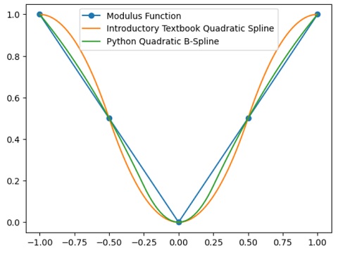
The picture shows the modulus function I used, with five data points one of which is at the origin (where there is a discontinuity in the first derivative). The orange curve is the result of the introductory textbook quadratic spline interpolation procedure, which does indeed perform quite badly with this pathological case. The green curve performs better and is the result of the in-built Python quadratic B-Spline method.

In producing the above picture, a default setting was used for the scipy.interpolate.BSpline() method and the question then arose as to whether the interpolation could be improved by adjusting the underlying B-Spline knot sequence. To experiment with this, I decided to replicate the in-built method using Python code which reveals more of the mathematical structure underlying B-Splines, and then to explore the effects of different knot settings.

B-Splines are a numerically convenient set of piecewise polynomial (pp) functions used as a basis for all other pp splines. Using standard notational conventions, a pp function $f$ of order $k$ is defined for $i = 1, \ldots, l$ as $f(x) = P_i(x)$ if $\xi_i < x < \xi_{i+1}$ , where $\xi = \{\xi_1, \ldots, \xi_{l+1}\}$ is a strictly increasing sequence of breakpoints and $P = \{P_1, \ldots, P_l\}$ is any sequence of polynomials of order $k$ (i.e., of degree $< k$ ). At each breakpoint other than $\xi_1$ and $\xi_{l+1}$ , the pp function is (arbitrarily) defined for computational purposes as taking the value from the right, i.e., $f(\xi_i) = f(\xi_i^{+})$ for $i = 2, \ldots, l$ . The collection of all pp functions of order $k$ with breakpoint sequence $\xi$ is a linear space of dimension $kl$ denoted by $\Pi_{<k, \xi}$ .

In general, it is necessary to impose continuity conditions on pp functions and their derivatives, of the form

$\text{jump}_{\xi_i} D^{j-1} f = 0$

for $j = 1, \ldots, \nu_i$ and $i = 2, \dots, l$ , where the notation means the jump of the function across the site $\xi_i$ , and $\nu = \{\nu_2, \nu_3, \dots, \nu_l\}$ is a set of nonnegative integers with $\nu_i$ counting the number of continuity conditions required at $\xi_i$ . (Note that there is no need for elements $\nu_1$ or $\nu_{l+1}$ in this list as continuity conditions are only needed to govern how different pieces of the pp function `meet’ at interior breakpoints). For example, $\nu_i = 2$ means that both the function and the first derivative are required to be continuous at $\xi_i$ , whereas $\nu_i = 0$ means that there are no continuity conditions at $\xi_i$ . The subset of all $f \in \Pi_{<k, \xi}$ satisfying the continuity conditions is a linear subspace of $\Pi_{<k, \xi}$ denoted by $\Pi_{<k, \xi;\nu}$ . The dimension of $\Pi_{<k, \xi;\nu}$ is

$n = kl - \sum_{i=2}^l \nu_i$

B-Splines originally emerged from the desire to have a numerically convenient basis for $\Pi_{<k, \xi;\nu}$ . To formally introduce B-Splines, let $t = {t_j}$ be a nondecreasing sequence of numbers (these are called `knots’ in the context of splines, and can be viewed as an extension of the breakpoint sequence $\xi$ defined earlier in the sense that $t$ can incorporate the elements of a given $\xi$ but does not have to be strictly increasing, and in principle it can be finite or infinite as required). Then the $j$ -th normalised B-Spline of order $k$ (i.e., of degree $k-1$ ) using knot sequence $t$ is denoted by $B_{j,k,t}$ , and its value at a site $x \in \mathbf{R}$ is given by

$B_{j,k,t}(x) = \frac{(x-t_j)B_{j,k-1,t}(x)}{t_{j+k-1} - t_j} + \frac{(t_{j+k} - x)B_{j+1,k-1,t}(x)}{t_{j+k} - t_{j+1}}$

This relation can be used to generate B-Splines by induction, starting from $B_{j,1,t}(x)$ , which is given by

$B_{j,1,t}(x) = \begin{cases} 1 & \text{if }t_j \leq x < t_{j+1}\\ 0 & \text{otherwise } \end{cases}$

Note that the B-Spline $B_{j,1,t}(x)$ is a piecewise polynomial of order $1$ and has support $[t_j, t_{j+1})$ , so it is continuous from the right in accordance with the convention for pp functions stated earlier. By putting $B_{j,1,t}(x)$ into the recurrence relation, we obtain the B-Spline $B_{j,2,t}(x)$ which is a piecewise polynomial of order $2$ with support $[t_j, t_{j+2})$ . B-Splines of higher order can be found via the recurrence relation in a convenient way using a tableau similar to the one commonly used to work out divided differences of functions.

A result known as the Curry-Schoenberg Theorem shows that the B-Splines as defined above constitute a basis for $\Pi_{<k, \xi;\nu}$ under certain conditions. Specifically, the theorem says that the sequence $\{B_{1,k,t}, B_{2,k,t}, \ldots, B_{n,k,t}\}$ is a basis for $\Pi_{<k, \xi;\nu}$ if:

(i) $\xi = \{\xi_1, \ldots, \xi_{l+1}\}$ is a strictly increasing sequence of breakpoints;

(ii) $\nu = \{\nu_2, \nu_3, \dots, \nu_l\}$ is a set of nonnegative integers with $\nu_i \leq k$ for all $i$ ;

(iii) $t = \{t_1, \ldots,t_{n+k}\}$ is a nondecreasing sequence with $n = kl - \sum_{i=2}^l \nu_i = \text{dim}\Pi_{<k, \xi;\nu}$ ;

(iv) for $i = 2, \ldots, l$ , the number $\xi_i$ occurs exactly $k - \nu_i$ times in $t$ ;

(v) $t_1 \leq t_2 \leq \ldots t_k \leq \xi_1$ and $\xi_{l+1} \leq t_{n+1} \leq \ldots \leq t_{n+k}$ .

These specifications provide the necessary information for generating a knot sequence $t$ from a given breakpoint sequence $\xi$ with the desired amount of `smoothness’ (i.e., number of continuity conditions), and we can then construct a B-Spline basis using the recurrence relation alluded to above. The number of continuity conditions at a breakpoint $\xi_i$ is determined by the number of times $\xi_i$ appears in $t$ , in the sense that each repetition of $\xi_i$ reduces the number of continuity conditions at that breakpoint by one. If $\xi_i$ appears $k$ times in $t$ , this corresponds to imposing no continuity conditions at $\xi_i$ . If $\xi_i$ appears $k-1$ times, the function is continuous at $\xi_i$ , but not its first or higher derivatives. If $\xi_i$ appears $k-2$ times, the function and its first derivative are continuous at $\xi_i$ , but not its second and higher derivatives; and so on. Note that a convenient choice of knot sequence is to make the first $k$ knot points equal to $\xi_1$ , and the last $k$ knot points equal to $\xi_{l+1}$ , thus imposing no continuity conditions at $\xi_1$ and $\xi_{l+1}$ .

Using this structure, I managed to replicate what the in-built scipy.interpolate.BSpline() method did above by using a breakpoint sequence

$\xi = \{-1, -0.25, 0.25, 1\}$

which is of length $l+1 = 4$ so the parameter $l$ is $3$ . The corresponding knot sequence is

$t = \{-1, -1, -1, -0.25, 0.25, 1, 1, 1\}$

The order is $k=3$ (corresponding to a degree $k-1 = 2$ for the polynomial pieces), and there are two continuity conditions for each of the interior points in the breakpoint sequence (the function and its first derivative are continuous) so using the standard notation we have $\nu = 4$ . The dimension of the subspace is thus $k l - v = 5$ so we expect to have five B-Splines in the basis set. In the picture below, I plot on the left the five basis B-Splines corresponding to $k=3$ and the above knot sequence, and on the right I show the resulting interpolation which is exactly the same as the one produced by the in-built scipy.interpolate.BSpline() method above:

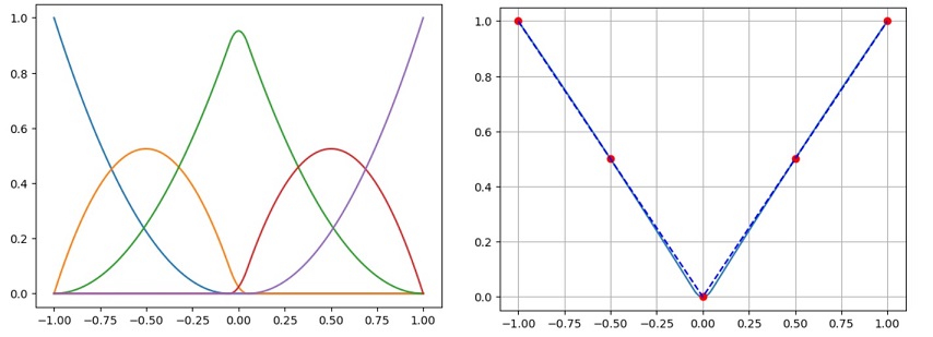
However, this is not the best we can do. The result can be improved substantially simply by adjusting the knot sequence a little. For example, an obvious adjustment would be to put the two interior knots much closer to the origin. I tried this with a new knot sequence

$t = \{-1, -1, -1, -0.05, 0.05, 1, 1, 1\}$

We still have five B-Splines in the basis set, but, as can be seen in the picture on the left below, the middle B-SPline has now become more `peaked’. The resulting interpolation shown on the right-hand side of the picture is now much better than the one produced by default using the scipy.interpolate.BSpline() method above:

So, this is a worked example of B-Splines allowing more flexibility to ‘fiddle with the settings’ in order to achieve a better quadratic spline interpolation.

Quadratic B-Spline interpolation of points on a modulus function

Published by Dr Christian P. H. Salas

Leave a comment Cancel reply