A max-flow/min-cut network problem solved both manually and with Python

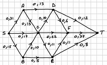
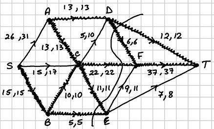
For a lecture on digraphs and network flows, I prepared the following capacitated directed network problem in order to explore its solution both manually via a maximum-flow/minimum-cut algorithm and computationally using the NetworkX library in Python:

The number on each arc represents the flow capacity of that arc and the vertices $S$ and $T$ are the source and the sink for the flow respectively (all arcs containing $S$ are directed away from $S$ and all arcs containing $T$ are directed towards $T$ ).

The max-flow/min-cut algorithm involves a labelling procedure which, starting from an initial flow (e.g., a zero flow) enables augmentation of flows along some arcs as well as reduction of flows along others. The idea is to increase the flow from $S$ to $T$ as much as possible subject to the capacity constraints on the arcs by using the algorithm to keep finding flow-augmenting routes through the network. The process terminates when all flow-augmenting routes have been found and a maximum flow value for the network thus becomes known. The algorithm will also result in some of the arcs in the network becoming saturated, i.e., filled to capacity, and a set of arcs containing some of these saturated arcs will constitute a minimum cut for the network. Such a minimum cut is a set of arcs with the smallest possible sum of capacities such that removal of all the arcs in the set divides the network into two disjoint parts $X$ and $Y$ , the part $X$ containing the source $S$ and the part $Y$ containing the sink $T$ . A theorem known as the max-flow min-cut theorem states that the maximum flow value must equal the capacity value of the minimum cut for a basic network such as the one in the diagram above. Finding a minimum cut using the saturated arcs at the end of the algorithm thus provides a useful way to check that the final flow is indeed a maximal one.

Below, I will solve the above problem both manually and using the NetworkX library in Python. For the manual solution, I will use a labelling procedure to record movement from one vertex $V$ to the next vertex $W$ with the notation $W(V, \varphi )$ , where $\varphi$ is the size of flow that is possible along the arc subject to the capacity of the arc and also subject to the possible flow at the previous step. Where there is a choice of arc when moving from one vertex to the next, we choose alphabetically. When moving backwards along an arc, this is indicated with a minus sign so that, for example, $V(W-, \varphi)$ indicates that we moved from $W$ to $V$ along an arc that was actually directed from $V$ to $W$ .

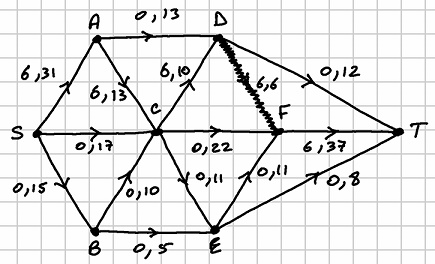
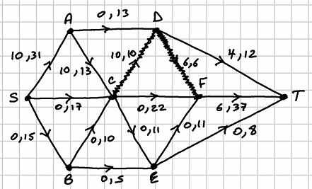
The manual solution is a little burdensome mainly because it requires making repeated copies of the network showing the adjustments at each step of the algorithm. Below I will render these copies by hand. At each step, each arc is labelled with two numbers separated by a comma, the first number being the flow along the arc and the second being the capacity of the arc. I will highlight that an arc is saturated by thickening the line representing the arc. We assume a zero initial flow, represented as follows in a manual copy of the above network:

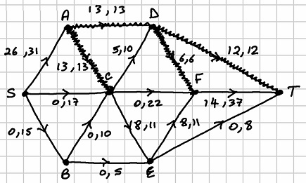
Starting from vertex $S$ , we choose alphabetically the arc $SA$ . The labels are: $A(S, 31) \ C(A, 13) \ D(C, 10) \ F(D, 6) \ T(F, 6)$ . The path is $SACDFT$ . The flow increase is $6$ . The saturated arc is $DF$ . Making these amendments, the network looks as follows after this first run:

For the next run, we begin again with arc $SA$ . The labels are: $A(S, 25) \ C(A, 7) \ D(C, 4) \ T(D, 4)$ . The path is $SACDT$ . The flow increase is $4$ . The saturated arc is $CD$ . The network looks as follows after this second run:

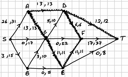
We begin again with arc $SA$ . The labels are: $A(S, 21) \ C(A, 3) \ E(C, 3) \ F(E, 3) \ T(F, 3)$ . The path is $SACEFT$ . The flow increase is $3$ . The saturated arc is $AC$ . The network looks as follows after this third run:

We begin again with arc $SA$ . The labels are: $A(S, 18) \ D(A, 13) \ T(D, 8)$ . The path is $SADT$ . The flow increase is $8$ . The saturated arc is $DT$ . The network looks as follows after this fourth run:

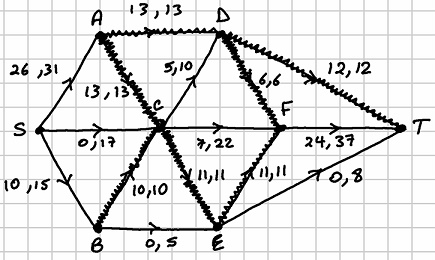
We begin again with arc $SA$ . The labels are: $A(S, 10) \ D(A, 5) \ C(D-, 5) \ E(C, 5) \ F(E, 5) \ T(F, 5)$ . The path is $SADCEFT$ . The flow increase is $5$ . The saturated arc is $AD$ . The network looks as follows after this fifth run:

Proceeding alphabetically, we now begin with arc $SB$ . The labels are: $B(S, 15) \ C(B, 10) \ E(C, 3) \ F(E, 3) \ T(F, 3)$ . The path is $SBCEFT$ . The flow increase is $3$ . The saturated arcs are $CE$ and $EF$ . The network looks as follows after this sixth run:

We begin again with arc $SB$ . The labels are: $B(S, 12) \ C(B, 7) \ F(C, 7) \ T(F, 7)$ . The path is $SBCFT$ . The flow increase is $7$ . The saturated arc is $BC$ . The network looks as follows after this seventh run:

We begin again with arc $SB$ . The labels are: $B(S, 5) \ E(B, 5) \ T(E, 5)$ . The path is $SBET$ . The flow increase is $5$ . The saturated arcs are $SB$ and $BE$ . The network looks as follows after this eighth run:

Proceeding alphabetically, we now begin with arc $SC$ . The labels are: $C(S, 17) \ F(C, 15) \ T(F, 13)$ . The path is $SCFT$ . The flow increase is $13$ . The saturated arc is $FT$ . The network looks as follows after this ninth run:

We begin again with arc $SC$ . The labels are: $C(S, 4) \ F(C, 2) \ E(F-, 2) \ T(E, 2)$ . The path is $SCFET$ . The flow increase is $2$ . The saturated arc is $CF$ . The network looks as follows after this tenth run:

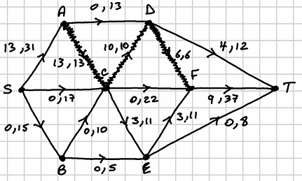
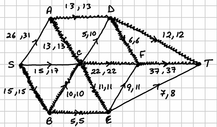
The algorithm is now complete. The diagram below shows the maximum flow and a minimum cut for this network:

The maximum flow has the value $26 + 15 + 15 = 56$ . The minimum cut is the set of arcs $(DT, DF, CF, CE, BE)$ which has capacity $12 + 6 + 22 + 11 + 5 = 56$ .

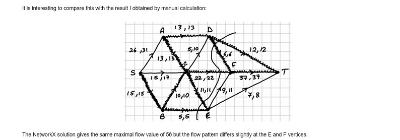
Having solved the problem manually, it is interesting to now compare this solution with a computational solution produced using the library NetworkX in Python. I did the coding for this problem in a Jupyter Notebook as follows: