On the equilibration of M/M/1 queues

The M/M/1 queue is the simplest Markov queueing model, and yet it is already sufficiently complicated to make it impractical in an introductory queueing theory lecture to derive time-dependent probability distributions for random variables of interest such as queue size and queueing time. A simpler approach is to assume the queue eventually reaches a steady state, and then use the forward Kolmogorov equations under this assumption to obtain equilibrium expected values of relevant random variables.

For the purposes of a lecture on this topic, I wanted to run some simulations of M/M/1 queues using Python to get a feel for how quickly or otherwise they actually reach their equilibrium. I was expecting equilibration after a few tens or hundreds of customers had passed through the queue. To my surprise, however, I ended up doing simulations involving a million customers and it typically took a few hundred thousand before the queue converged to theoretically predicted equilibrium values of things like mean queue size and mean queueing time. I want to record the relevant calculations and Python simulations here.

In M/M/1 queues, arrivals of customers occur according to a Poisson process with rate $\lambda$ , there is a single server, and departures occur according to a Poisson process with rate $\epsilon$ (so, the service time for each customer is exponentially distributed, also with rate $\epsilon$ ). Suppose the queue contains $x$ customers at time $t + \delta t$ where $\delta t$ is a small time increment. Given the axioms of a Poisson process, there are only three possibilities for the number of customers at time $t$ :

There could have been $x + 1$ customers at time $t$ and one departed, or there could have been $x - 1$ customers at time $t$ and one arrived, or there could have been $x$ customers at time $t$ and there were no departures or arrivals. By the axioms of a Poisson process, these three possibilities have probabilities

$p_{x + 1, x}(t, t + \delta t) = \epsilon \delta t + o(\delta t)$

$p_{x - 1, x}(t, t + \delta t) = \lambda \delta t + o(\delta t)$

$p_{x, x}(t, t + \delta t) = 1 - (\lambda + \epsilon) \delta t + o(\delta t)$

for the cases $x = 1, 2, 3, \dots$ . In the case $x = 0$ , we have

$p_{- 1, 0}(t, t + \delta t) = 0$

$p_{0, 0}(t, t + \delta t) = 1 - \lambda \delta t + o(\delta t)$

since a departure is impossible when there are no customers in the queue.

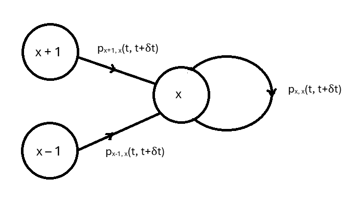
The M/M/1 queue is a continuous-time Markov process for which Chapman-Kolmogorov equations can be obtained by applying the Theorem of Total Probability. The Chapman-Kolmogorov equations say that

$p_{i, x}(0, t + \delta t) = \sum_k p_{i, k}(0, t) p_{k, x}(t, t + \delta t)$

where $i$ is the number of customers at time 0 and the summation is over all relevant states $k$ in the state space. The only relevant states $k$ here are $x + 1$ , $x - 1$ , and $x$ as outlined above, so the Chapman-Kolmogorov equations for the current situation are

$p_{i, x}(0, t + \delta t) = p_{i, x}(0, t) p_{x, x}(t, t + \delta t)$

$+ p_{i, x - 1}(0, t) p_{x - 1, x}(t, t + \delta t) + p_{i, x + 1}(0, t) p_{x + 1, x}(t, t + \delta t)$

$= p_{i, x}(0, t) (1 - (\lambda + \epsilon) \delta t) + p_{i, x - 1}(0, t) \lambda \delta t + p_{i, x + 1}(0, t) \epsilon \delta t$

Rearranging, we get

$\frac{p_{i, x}(0, t + \delta t) - p_{i, x}(0, t)}{\delta t}$

$= \lambda p_{i, x - 1}(0, t) + \epsilon p_{i, x + 1}(0, t) - (\lambda + \epsilon) p_{i, x}(0, t) + \frac{o(\delta t)}{\delta t}$

Letting $\delta t \rightarrow 0$ , we get the Kolmogorov forward equations for the M/M/1 queue:

$\frac{d}{dt} p_{i, x}(0, t) = \lambda p_{i, x - 1}(0, t) + \epsilon p_{i, x + 1}(0, t) - (\lambda + \epsilon) p_{i, x}(0, t)$

for the cases $x = 1, 2, 3, \dots$ , and

$\frac{d}{dt} p_{i, 0}(0, t) = \epsilon p_{i, 1}(0, t) - \lambda p_{i, 0}(0, t)$

for the case $x = 0$ .

These equations can be solved to get a time-dependent probability distribution for the queue size, but the procedure is far from straightforward and the time-dependent probability distribution itself is very complicated. What can be done far more easily is to assume that the process reaches a steady state after many customers have arrived and departed, and then calculate the expected values of random variables of interest such as the expected queue size and the expected queueing time. This is what we will do here, before confirming the calculations using Python simulations.

When the process has reached a steady state, the probabilities $p_{i, x}(0, t)$ are no longer changing over time, so we have $\frac{d}{dt} p_{i, x}(0, t) = 0$ . Setting the left-hand sides of the Kolmogorov forward equations equal to zero and solving the equations recursively for $x = 0$ and then $x = 1, 2, 3, \ldots$ , we get

$p_{i, x} = \big(\frac{\lambda}{\epsilon} \big)^x \cdot p_{i, 0}$

for $x = 0, 1, 2, \ldots$ , where $\lambda/\epsilon$ is called the traffic intensity. For the equilibrium distribution to exist, these probabilities must sum to 1, which requires $\lambda/\epsilon < 1$ . In this case, we have

$\sum_x \big(\frac{\lambda}{\epsilon} \big)^x \cdot p_{i, 0} = \frac{p_{i, 0}}{1 - \big(\frac{\lambda}{\epsilon} \big)} = 1$

so,

$p_{i, 0} = 1 - \big(\frac{\lambda}{\epsilon} \big)$

Substituting this into the equation for $p_{i, x}$ above we get

$p_{i, x} = \big(1 - \big(\frac{\lambda}{\epsilon} \big) \big) \big(\frac{\lambda}{\epsilon} \big)^x$

which is the probability mass function of a geometric distribution starting at 0 with parameter $\lambda/\epsilon$ . The mean queue size in the steady state of this process is the mean of this distribution, which is

$\frac{\big(\frac{\lambda}{\epsilon} \big)}{1 - \big(\frac{\lambda}{\epsilon} \big)}$

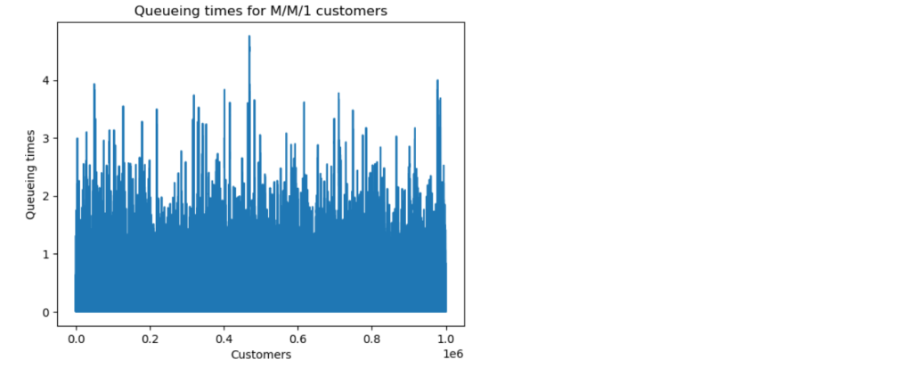
It can also be shown fairly straightforwardly that the mean queueing time for the M/M/1 queue in equilibrium is the mean of an exponential distribution with parameter $\epsilon - \lambda$ , so the mean queueing time is

$\frac{1}{\epsilon - \lambda}$

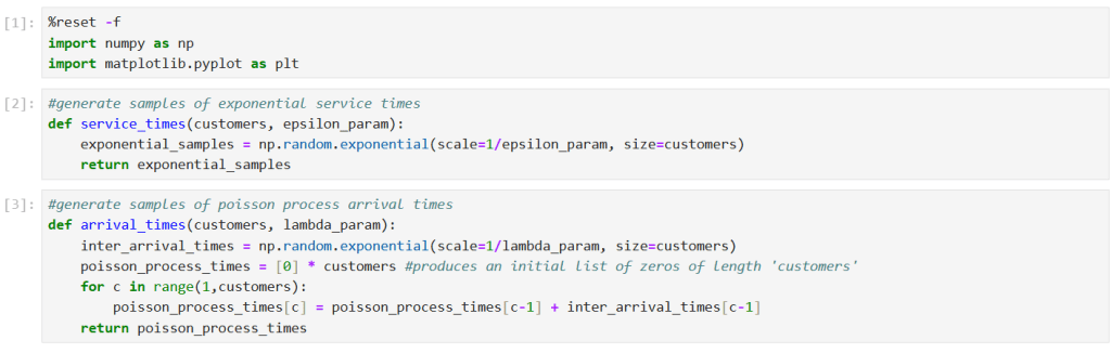
To simulate this M/M/1 queue in Python, we begin by defining Python functions for the exponential service times and Poisson arrivals:

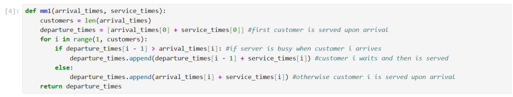
Next, we compute departure times for customers in an M/M/1 queue given the arrival times and service times generated by the previous functions. Each customer is either served upon arrival if the server is free, or has to wait for the previous customer to depart before being served.

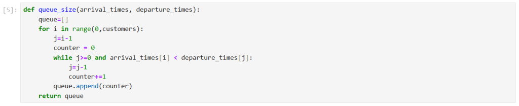
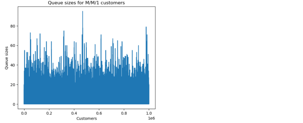
We can also compute queue sizes, given the arrival times and departure times of customers. To clarify the algorithm, suppose we want to know the queue size when customer 5 arrives. We set counter = 0 to initialise it and we set j = 4 to look at customer 4’s departure time. If the arrival time of customer 5 is before the departure time of customer 4, then we know there was at least one person in the queue so we set counter = 1 and change j = 3 to look at customer 3’s departure time. We continue with this process until the arrival time of customer 5 is after the departure time of a previous customer, or until we reach j = 0 at which point we will have counter = 4 if the arrival time of customer 5 is before the departure time of customer 0. We will then set j = -1 and the counting process will stop.

We can now run a simulation. The results below are for a simulation with one million customers, and parameter values $\lambda = 18$ and $\epsilon = 20$ . The predicted equilibrium mean queueing time is $1/(20 - 18) = 0.5$ time units, and the predicted equilibrium mean queue size is $(18/20)/(1 - (18/20)) = 9$ .

We now explore how long it takes for the M/M/1 queue to settle down to its steady state. We look at the convergence of both the queueing time means and the queue size means to their theoretical equilibrium values.

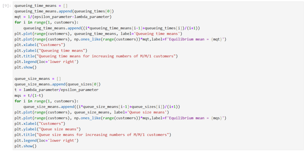
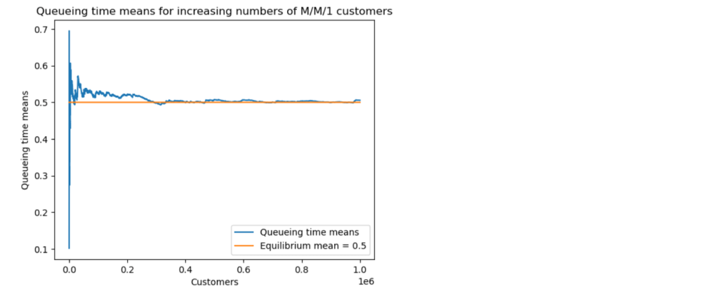
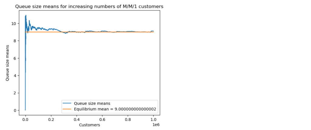
The simulation with one million customers eventually settled down to the predicted theoretical values for mean queue size and mean queueing time, but this took a surprisingly long time, around 400 thousand customers.

On the equilibration of M/M/1 queues

Published by Dr Christian P. H. Salas

Leave a comment Cancel reply