Python simulation of a threshold phenomenon in a general epidemic

For a lecture on deterministic and stochastic general epidemic models, I ran a Python simulation illustrating a threshold phenomenon which determines how an epidemic evolves. I want to record the results of this here.

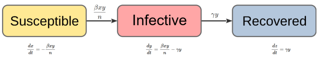
In a general epidemic model, we assume a closed community of $n + 1$ individuals and classify those individuals into three groups, those who are susceptible to disease, those who are infective, and those who are removed (i.e., who have had the disease and are no longer infective). The numbers of each type at time $t$ are denoted by $X(t)$ , $Y(t)$ and $Z(t)$ respectively. Note that since $Z(t) = n + 1 - (X(t) + Y(t))$ , the time evolution of $Z(t)$ is automatically determined by the evolution of $X(t)$ and $Y(t)$ . At any given time $t$ , only two types of transition are possible. The first type of transition is SUSCEPTIBLE $\rightarrow$ INFECTIVE in which an infective meets a susceptible and the disease is passed on, causing the number of susceptibles to decrease by one and the number of infectives to increase by one. The second type of transition is INFECTIVE $\rightarrow$ REMOVED in which an infective recovers from the disease, so the total number of infectives decreases by one and the total number removed increases by one.

Assuming that each member of the community comes into contact with the remaining $n$ others according to a Poisson process with rate $\beta$ , that there is homogenous mixing so that the probability of one member meeting any other particular member is $1/n$ , and that a susceptible who becomes infected with the disease only remains infective for a time drawn from an exponential distribution with rate $\gamma$ , then the general epidemic as a stochastic process can be characterised by the following two probability statements corresponding to the two types of transitions outlined above:

$P(X(t + \delta t) = x - 1, Y(t + \delta t) = y + 1 | X(t) = x, Y(t) = y)$

$= \frac{\beta x y}{n} \delta t + o(\delta t) \quad \quad \quad \quad (1)$

$P(X(t + \delta t) = x, Y(t + \delta t) = y - 1 | X(t) = x, Y(t) = y)$

$= \gamma y \delta t + o(\delta t) \quad \quad \quad \quad (2)$

The first probability statement says that infectives meet susceptibles according to a Poisson process with rate $\beta x y/n$ , while the second probability statement says that infectives recover and become removed according to a Poisson process with rate $\gamma y$ , where $x$ and $y$ denote realised numbers of susceptibles and infectives at time $t$ respectively.

To obtain a deterministic approximation of the above stochastic general epidemic model, we set up ordinary differential equations for the time evolution of $x$ , $y$ and $z$ based on the probability statements (1) and (2). From (1), we see that susceptibles $x$ decrease at the rate $\beta x y/n$ and infectives $y$ correspondingly increase at the same rate, while from (2) we see that infectives also decrease at the rate $\gamma y$ and the removed $z$ correspondingly increase at the same rate. We thus get the following system of three coupled ordinary differential equations for the deterministic general epidemic model:

$\frac{dx}{dt} = -\frac{\beta x y}{n} \quad \quad \quad \quad (3)$

$\frac{dy}{dt} = \frac{\beta x y}{n} - \gamma y \quad \quad \quad \quad (4)$

$\frac{dz}{dt} = \gamma y \quad \quad \quad \quad (5)$

These cannot generally be solved to get explicit expressions for $x$ , $y$ and $z$ as functions of time, but can be solved numerically to get time paths for these variables, as shown below using Python. It is also straightforward to obtain a differential equation for $y$ in terms of $x$ by dividing (4) by (3) to get

$\frac{dy}{dx} = \frac{dy/dt}{dx/dt} = \frac{\frac{\beta x y}{n} - \gamma y}{-\frac{\beta x y}{n}} = \frac{\rho - x}{x} \quad \quad \quad \quad (6)$

where

$\rho = \frac{n \gamma}{\beta} \quad \quad \quad \quad (7)$

is a key parameter known as the epidemic parameter. The differential equation (6) can easily be solved given initial conditions $x(0) = x_0$ , $y(0) = y_0$ , $z(0) = z_0$ , to get an equation for $y$ in terms of $x$ :

$y - y_0 = (x_0 - x) - \rho \ln \bigg( \frac{x_0}{x}\bigg) \quad \quad \quad \quad (8)$

This equation describes the evolution of the epidemic in a `timeless’ way in the $(x, y )$ -plane and predicts that the epidemic parameter $\rho$ plays a crucial role. It acts as a threshold parameter in the following sense: if $x_0 \leq \rho$ , the number of infectives never rises above the initial number $y_0$ and in fact declines steadily from there until it reaches $y = 0$ at which point the epidemic ends (since there are no more infectives to pass on the disease), whereas if $x_0 > \rho$ , the number of infectives can rise significantly above $y_0$ until it reaches a maximum value before beginning to decline from there until the epidemic ends again when $y = 0$ . Public health measures therefore aim to reduce the number of susceptibles $x_0$ (e.g., by immunisation) and to increase the value of the epidemic parameter $\rho$ by increasing the removal rate $\gamma$ and decreasing the contact rate $\beta$ (e.g., by encouraging self-isolation) to try to achieve a scenario in which $x_0 < \rho$ .

To supplement these results, I wanted to use Python to get time paths for $x$ , $y$ and $z$ as direct numerical solutions to the coupled differential equations (3), (4) and (5), ideally also demonstrating the threshold phenomenon with these time paths. The following diagram summarises the deterministic general epidemic model to be implemented in Python:

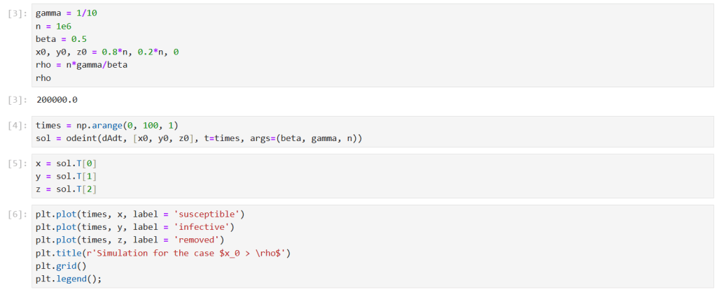
I used the odeint() function from the scipy.integrate library to solve the differential equation system numerically. This requires the definition of a Python function which takes as inputs $\mathbf{A} = (x, y, z)$ , $t$ , $\beta$ , $\gamma$ and $n$ , and returns the vector derivative $d \mathbf{A}/dt = (dx/dt, dy/t, dz/dt)$ .

First, I ran a simulation for the case $x_0 > \rho$ . I solved the model equations for

$\gamma = 1/10~\mathrm{ days^{-1}}$
$n=1.0 \times 10^6$
$\beta = 0.5~\mathrm{ days^{-1}}$
$(x_0, y_0, z_0) = (0.8 \times n, 0.2 \times n, 0)$

Note that the corresponding epidemic parameter is $\rho = n \gamma/\beta = 200000$ .

The results show the classic epidemic pattern for $x_0 > \rho$ , with the number of infectives rising significantly above $y_0$ before declining to $y = 0$ . Note that almost all the susceptibles ended up being infected in this scenario.

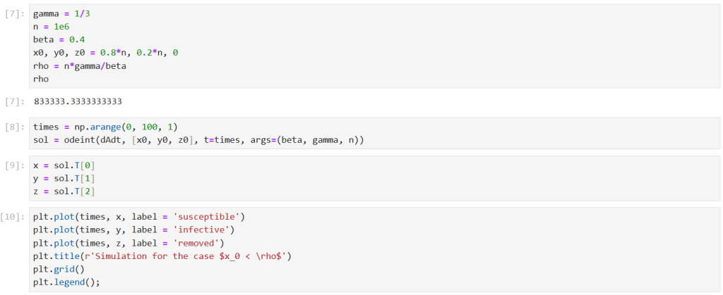
Next, I ran a simulation for the case $x_0 < \rho$ . Suppose that public health measures have managed to increase the value of the epidemic parameter $\rho$ by increasing the removal rate $\gamma$ and reducing the contact rate $\beta$ . I solved the model equations for

$\gamma = 1/3~\mathrm{ days^{-1}}$
$n=1.0 \times 10^6$
$\beta = 0.4~\mathrm{ days^{-1}}$
$(x_0, y_0, z_0) = (0.8 \times n, 0.2 \times n,0)$

Note that the corresponding epidemic parameter is now $\rho = n \gamma / \beta = 833333.333...$ .

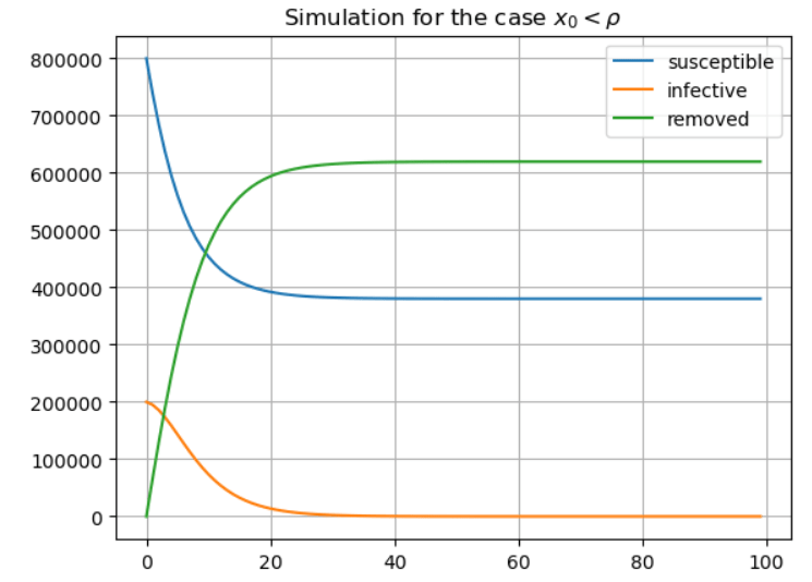
The results now show the typical results for $x_0 < \rho$ , with the number of infectives never rising above the initial $y_0$ , and declining steadily to $y = 0$ . Note that almost half of the initial number of susceptibles remained unaffected by the disease in this scenario.

Python simulation of a threshold phenomenon in a general epidemic

Published by Dr Christian P. H. Salas

Leave a comment Cancel reply