The following is a record of some notes I made on the main mathematical developments in Michael Wilkinson’s 2016 Physical Review Letter on the large deviation analysis of rapid-onset rain showers (reference: Wilkinson, M., 2016, Large Deviation Analysis of Rapid Onset of Rain Showers, Phys. Rev. Lett. 116, 018501). This publication will be referred to as MW2016 herein. The published Letter has an accompanying Supplement which will also be referred to here. The Supplement provides additional details of some intricate derivations underlying key results presented in the main Letter.
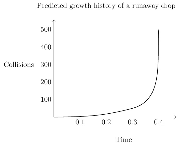
One of the main contributions of MW2016 is that it shows that large deviation theory is the correct framework for analysing the implications of a collector-drop model of rapid rain formation which was discussed in a previous paper by Kostinski and Shaw (reference: Kostinski, A., Shaw, R., 2005, Fluctuations and Luck in Droplet Growth by Coalescence, Bull. Am. Meteorol. Soc. 86, 235). In this collector-drop model, a runaway droplet falls and coalesces at a rapidly increasing rate with many smaller water particles. The collision rates are assumed to increase according to a simple power law function of the number of collisions. In addition to formulating a volume fraction cut-off mechanism for raindrop size, MW2016 also successfully uses large deviation analysis in conjunction with asymptotic approximations to study the link between the time scale for rapid onset of rain showers and the number of water particle collisions needed for raindrop formation. In the present article, I provide a mathematical review of the key points in MW2016 and also detail some errata in the published Letter which were identified in the review process.
Mathematical review
In the collector-drop model, a runaway droplet falls and collides with a large number  of small droplets of radius
  according to an inhomogeneous Poisson process. If the random variable
  represents the inter-collision time leading up to the
  -th collision, the time for a droplet to experience runaway growth is then the random variable

The inter-collision times are independent exponentially distributed random variables with

where  is the number of collisions per second, i.e., the collision rate, by the time of the -th collision. The collision rate is modelled as

where

is the collision rate of a drop of radius  with droplets of radius . Here,
  is the coalescence efficiency,
  is the number density of microscopic water droplets per
  ,
,  is the effective cross-section area and
  is the relative velocity. The constant
  is a constant of proportionality between terminal velocity and the radius squared of a water particle.
The function  in (3) characterises the dependence of on the number of collisions. In the Kostinski and Shaw 2005 paper referenced above,
  , but we can have
  when
when  and
and  . MW2016 treats as a simple power law, so that

The average inter-collision time leading to the -th collision is then given by

and the mean time for explosive growth is obtained as

When  , the mean time for explosive growth converges as
  , giving

where  is Riemann’s zeta function.
A cut-off mechanism for raindrop size is obtained by considering the liquid water content of a cloud, expressed as a volume fraction  . Since is the number of water particles of radius per , and each particle is a sphere with volume
  , the volume fraction of liquid water per of cloud is given by

For example, if each droplet is initially of radius  , and there are
  such droplets per of cloud, then
  .
.
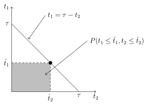
Using (2), the fraction of droplets undergoing runaway growth between times  and
and  is given by

For example, if  , then `one in a million’ water droplets will undergo runaway growth between times and .
If the volume of each runaway droplet increases by a factor of , the volume fraction of liquid water removed from the cloud per over the time interval of length  will then be

For example, if  , and , then the volume fraction of liquid water content per is reduced by
  over the time interval of length . This represents a
  per cent reduction in .
As  , the instantaneous change of the liquid water content of a cloud per due to runaway growth of droplets is thus

Therefore, the instantaneous percentage rate of decline of the volume fraction is

Integrating (13) over a time interval then gives a percentage loss  in that interval:

The onset of a shower is determined by the criterion that be a significant percentage of the liquid water content of a cloud that is removed by raindrop formation as a result of particle collisions. We are now interested in finding the time scale  over which this significant reduction in occurs. In accordance with (14), this satisfies

where  .
.
To make progress from here, MW2016 approximates  in (15) using the large deviation principle, which is explained in detail in, e.g., an article by Touchette (reference: Touchette, H., 2009, The large deviation approach to statistical mechanics, Phys. Rep. 478, 1). With
  defined as in (1) and
  given by (7), we implement the large deviation principle here by approximating the probability
  at some value
  in the small-value tail of the distribution of as
![P(\bar{T})d\bar{T} = P(T \in [\bar{T}, \bar{T} + d\bar{T}])](https://s0.wp.com/latex.php?latex=P%28%5Cbar%7BT%7D%29d%5Cbar%7BT%7D+%3D+P%28T+%5Cin+%5B%5Cbar%7BT%7D%2C+%5Cbar%7BT%7D+%2B+d%5Cbar%7BT%7D%5D%29&bg=ffffff&fg=111111&s=0&c=20201002)
where  is given by
![P(\bar{T}) = \frac{1}{\langle T \rangle} \exp[-J(\tau)] \quad \quad \quad \quad \quad (16)](https://s0.wp.com/latex.php?latex=P%28%5Cbar%7BT%7D%29+%3D+%5Cfrac%7B1%7D%7B%5Clangle+T+%5Crangle%7D+%5Cexp%5B-J%28%5Ctau%29%5D+%5Cquad+%5Cquad+%5Cquad+%5Cquad+%5Cquad+%2816%29&bg=ffffff&fg=111111&s=0&c=20201002)
with  . The function
  in (16) is referred to as an entropy function or rate function in large deviation theory, and is defined below. Using (16) in (15) we get the condition for the onset of rainfall as
![\mathcal{N^{*}} \int_0^{t^{*}} \frac{d \bar{T}}{\langle T \rangle} \exp \bigg[-J\bigg(\frac{\bar{T}}{\langle T \rangle}\bigg)\bigg] = \mathcal{N^{*}} \int_0^{t^{*}} d \tau^{\prime} \exp [-J(\tau^{\prime})] = 1 \quad \quad \quad \quad \quad (17)](https://s0.wp.com/latex.php?latex=%5Cmathcal%7BN%5E%7B%2A%7D%7D+%5Cint_0%5E%7Bt%5E%7B%2A%7D%7D+%5Cfrac%7Bd+%5Cbar%7BT%7D%7D%7B%5Clangle+T+%5Crangle%7D+%5Cexp+%5Cbigg%5B-J%5Cbigg%28%5Cfrac%7B%5Cbar%7BT%7D%7D%7B%5Clangle+T+%5Crangle%7D%5Cbigg%29%5Cbigg%5D+%3D+%5Cmathcal%7BN%5E%7B%2A%7D%7D+%5Cint_0%5E%7Bt%5E%7B%2A%7D%7D+d+%5Ctau%5E%7B%5Cprime%7D+%5Cexp+%5B-J%28%5Ctau%5E%7B%5Cprime%7D%29%5D+%3D+1+%5Cquad+%5Cquad+%5Cquad+%5Cquad+%5Cquad+%2817%29&bg=ffffff&fg=111111&s=0&c=20201002)
with  . A saddle-point approximation for the integral here at the maximum value of the integrand,
 ![\exp[-J(\tau^{*})]](https://s0.wp.com/latex.php?latex=%5Cexp%5B-J%28%5Ctau%5E%7B%2A%7D%29%5D&bg=ffffff&fg=111111&s=0&c=20201002) , with
, with  , then gives the condition for the onset of rainfall as
![\mathcal{N}^{*} \exp[-J(\tau^{*})] = 1 \quad \quad \quad \quad \quad (18)](https://s0.wp.com/latex.php?latex=%5Cmathcal%7BN%7D%5E%7B%2A%7D+%5Cexp%5B-J%28%5Ctau%5E%7B%2A%7D%29%5D+%3D+1+%5Cquad+%5Cquad+%5Cquad+%5Cquad+%5Cquad+%2818%29&bg=ffffff&fg=111111&s=0&c=20201002)
Taking logs, we can write the condition alternatively as

What is required now is to find an expression for  in terms of
  , using (19). To obtain this, it is necessary to find an expression for the rate function for the random sum defined by (1) and (2).
Consider a single inter-collision time with density (2). Following the approach in the article by Touchette cited above for the purposes of the large deviation analysis here, we obtain the log of the Laplace transform of the random variable , often referred to as its scaled cumulant generating function, as

To ensure the logarithm on the right-hand side is always defined, we need to restrict the admissible values of  to the interval
  . Inter-collision times are assumed to be independent, so for a sum of inter-collision times such as (1), we get the log of the Laplace transform of as


This is differentiable with respect to for all  , so by the Gartner-Ellis Theorem of large deviation analysis, discussed in Touchette, the rate function in (16) is given by

The expression on the right-hand side of (22) is referred to as the Fenchel-Legendre transform of  .
.
Note that the expression in (22) is the negative of the expression usually given in large deviation theory. This is because the outer function in the formulation of the log of the Laplace transform in (20) above is the negative of the expression used, e.g., in Touchette, and this formulation also has the parameter negated. The alternative formulation would be

and the associated entropy function for this would then be the more conventional

In this case, the admissible values of would be those in the interval  . Essentially, the signs of and have been negated in the formulation in MW2016, as this is more convenient for the analysis.
Differentiating the bracketed expression in (22) with respect to and setting equal to zero we obtain

But

Putting this in (23) we get

This implicitly gives an optimal value of as a function of  , say
, say  . If this could be obtained explicitly, inserting it into the right-hand side of (22) would give the required rate function :

However, in practice it is not possible to obtain an exact expression for in this way. Instead, MW2016 obtains asymptotic expressions for which are valid for small . This is achieved by reparameterising using a scaled variable  , defined as

From (7) and (8) we get, as ,

Using (5), (27) and (28) in (25) we get

The expression on the right-hand side of (29) appears in equation (18) in MW2016.
We now write (2.21) in reparameterised form as as

We also write

Then we re-express (26) in the form

This appears as equation (19) in MW2016.
Following the approach in the Supplement to MW2016, the next stage in the development is to obtain an asymptotic expression for the sum in (30) as  . (It is assumed from now on that
  , to simplify the expressions). Upon differentiating this, we will then obtain a corresponding asymptotic expression for in accordance with (29), which can be inverted to obtain a small approximation for , and subsequently a small approximation for
  . Finally, this will be used in (19) to obtain an expression for in terms of
  .
.
Begin by approximating the sum in (30) as an integral. Observe that


(The third line is obtained by making the change of variable  in each integral in the second line, with
  representing the fixed positive integer in the upper limit, so
  , and
, and  when
when  whereas
  when
when  ). Therefore


In MW2016 this is written as

where


Write  . Then as
  we have


Therefore, when  , we can approximate each
  by using


When  but is not necessarily large, we can write
![\triangle S_n \sim \int_0^1 dx \ln[\kappa n^{-\gamma}(1 + n^{\gamma}/\kappa)] - \int_0^1 dx \ln[\kappa (n-x)^{-\gamma}(1 + (n - x)^{\gamma}/\kappa]](https://s0.wp.com/latex.php?latex=%5Ctriangle+S_n+%5Csim+%5Cint_0%5E1+dx+%5Cln%5B%5Ckappa+n%5E%7B-%5Cgamma%7D%281+%2B+n%5E%7B%5Cgamma%7D%2F%5Ckappa%29%5D+-+%5Cint_0%5E1+dx+%5Cln%5B%5Ckappa+%28n-x%29%5E%7B-%5Cgamma%7D%281+%2B+%28n+-+x%29%5E%7B%5Cgamma%7D%2F%5Ckappa%5D&bg=ffffff&fg=111111&s=0&c=20201002)

and we can ignore the  component as . Next, make the change of variable
  in the integral in (36). Then when ,
  , when ,
  , and
, and  . We get


![= -\gamma\bigg[(n-1) \ln\bigg(\frac{n-1}{n}\bigg)+ 1\bigg] \quad \quad \quad \quad \quad (37)](https://s0.wp.com/latex.php?latex=%3D+-%5Cgamma%5Cbigg%5B%28n-1%29+%5Cln%5Cbigg%28%5Cfrac%7Bn-1%7D%7Bn%7D%5Cbigg%29%2B+1%5Cbigg%5D+%5Cquad+%5Cquad+%5Cquad+%5Cquad+%5Cquad+%2837%29&bg=ffffff&fg=111111&s=0&c=20201002)
In order to evaluate  using (33), MW2016 splits the summation over into two parts: choose an integer
  such that
  and let
  as . Use (35) for when
  , and (37) when
  . We get
![S \sim S_0 - \gamma \sum_{n=1}^M \bigg[(n-1) \ln\bigg(\frac{n-1}{n}\bigg)+ 1\bigg] - \gamma \kappa \sum_{n = M+1}^{\infty} \frac{1}{2n(\kappa + n^{\gamma})} \quad \quad \quad \quad \quad (38)](https://s0.wp.com/latex.php?latex=S+%5Csim+S_0+-+%5Cgamma+%5Csum_%7Bn%3D1%7D%5EM+%5Cbigg%5B%28n-1%29+%5Cln%5Cbigg%28%5Cfrac%7Bn-1%7D%7Bn%7D%5Cbigg%29%2B+1%5Cbigg%5D+-+%5Cgamma+%5Ckappa+%5Csum_%7Bn+%3D+M%2B1%7D%5E%7B%5Cinfty%7D+%5Cfrac%7B1%7D%7B2n%28%5Ckappa+%2B+n%5E%7B%5Cgamma%7D%29%7D+%5Cquad+%5Cquad+%5Cquad+%5Cquad+%5Cquad+%2838%29&bg=ffffff&fg=111111&s=0&c=20201002)
We now approximate the second summation using an integral:

Make the change of variable  . Then
  , so
, so  , and when
  ,
,  , while when
  ,
,  . The integral in (39) becomes


![= -\frac{1}{2} \ln \bigg[\kappa M^{-\gamma} \bigg(1 + \frac{1}{\kappa M^{-\gamma}}\bigg)\bigg]](https://s0.wp.com/latex.php?latex=%3D+-%5Cfrac%7B1%7D%7B2%7D+%5Cln+%5Cbigg%5B%5Ckappa+M%5E%7B-%5Cgamma%7D+%5Cbigg%281+%2B+%5Cfrac%7B1%7D%7B%5Ckappa+M%5E%7B-%5Cgamma%7D%7D%5Cbigg%29%5Cbigg%5D&bg=ffffff&fg=111111&s=0&c=20201002)


Putting this in (38) we get
![S \sim S_0 - \gamma \sum_{n=1}^M \bigg[(n-1) \ln\bigg(\frac{n-1}{n}\bigg)+ 1\bigg] -\frac{1}{2} \ln(\kappa) + \frac{\gamma}{2} \ln(M) + O(\kappa^{-1}) \quad \quad \quad \quad \quad (40)](https://s0.wp.com/latex.php?latex=S+%5Csim+S_0+-+%5Cgamma+%5Csum_%7Bn%3D1%7D%5EM+%5Cbigg%5B%28n-1%29+%5Cln%5Cbigg%28%5Cfrac%7Bn-1%7D%7Bn%7D%5Cbigg%29%2B+1%5Cbigg%5D+-%5Cfrac%7B1%7D%7B2%7D+%5Cln%28%5Ckappa%29+%2B+%5Cfrac%7B%5Cgamma%7D%7B2%7D+%5Cln%28M%29+%2B+O%28%5Ckappa%5E%7B-1%7D%29+%5Cquad+%5Cquad+%5Cquad+%5Cquad+%5Cquad+%2840%29&bg=ffffff&fg=111111&s=0&c=20201002)
We can write this as
![S \sim S_0 - \gamma \bigg\{\sum_{n=1}^M \bigg[(n-1) \ln\bigg(\frac{n-1}{n}\bigg)+ 1\bigg] - \frac{1}{2} \ln(M)\bigg\}](https://s0.wp.com/latex.php?latex=S+%5Csim+S_0+-+%5Cgamma+%5Cbigg%5C%7B%5Csum_%7Bn%3D1%7D%5EM+%5Cbigg%5B%28n-1%29+%5Cln%5Cbigg%28%5Cfrac%7Bn-1%7D%7Bn%7D%5Cbigg%29%2B+1%5Cbigg%5D+-+%5Cfrac%7B1%7D%7B2%7D+%5Cln%28M%29%5Cbigg%5C%7D&bg=ffffff&fg=111111&s=0&c=20201002)

Taking the limit as , the term in curly brackets in (41) converges to a constant  , and we get

This is equation [10] in the Supplement to MW2016.
From (29), we see that differentiating  in (30) gives a time
  . The corresponding asymptotic expression for
  is obtained by differentiating (42). We get

In the integral in (43), make the change of variable  , so that
  . Then

The integral in (43) then becomes

so we get

with

(MW2016 notes that the integral in (45) is actually the beta function  ). Integrating the first term on the right-hand side of (44), which is
  , gives

Substituting for  in (42) with the expression in (46) gives

This is equation (21) in MW2016.
To obtain an explicit expression for the rate function , we must now invert (44) to express the parameter in terms of the time , and hence in terms of the dimensionless time given by  . To this end, observe that from (44) we get

Therefore

so

with  . Now, using (47) and (48), the rate function is given by


Using (49) in (50) we get

where  is another constant.
We are now finally in a position to obtain the result given in (27) in MW2016. From (51) we see that to leading order we have
![J(\tau^{*}) \propto [\tau^{*}]^{-\frac{1}{\gamma-1}}](https://s0.wp.com/latex.php?latex=J%28%5Ctau%5E%7B%2A%7D%29+%5Cpropto+%5B%5Ctau%5E%7B%2A%7D%5D%5E%7B-%5Cfrac%7B1%7D%7B%5Cgamma-1%7D%7D&bg=ffffff&fg=111111&s=0&c=20201002)
so from (19) we obtain
![\tau^{*} \propto [\ln \mathcal{N}^{*}]^{-(\gamma - 1)} \quad \quad \quad \quad \quad (52)](https://s0.wp.com/latex.php?latex=%5Ctau%5E%7B%2A%7D+%5Cpropto+%5B%5Cln+%5Cmathcal%7BN%7D%5E%7B%2A%7D%5D%5E%7B-%28%5Cgamma+-+1%29%7D+%5Cquad+%5Cquad+%5Cquad+%5Cquad+%5Cquad+%2852%29&bg=ffffff&fg=111111&s=0&c=20201002)
Errata in MW216
In the course of working with MW2016, some errata have come to light which I will record here.
In a private written communication with Michael Wilkinson, I pointed out that an error was made in the Supplement to MW2016 which details the asymptotic analysis. The issue arises in the Supplement when combining equations (17) and (19) there to get equation (20), which is then presented as equation (24) in the main MW2016 text. Equation (17) for in the Supplement has a leading order term involving the dimensionless time variable with an exponent of the form  . Using (17) in equation (19) for the entropy, we should get the leading order term appearing with exponent
  , because in (19) appears raised to the power
  . However, the exponent is incorrectly given as . This error affected the time scale relationship reported in (27) in the main MW2016 text. Combining the expression for the entropy with the condition (12) in the main MW2016 text for the onset of a shower, should be related to
  with an exponent
  on the latter, i.e., the reciprocal of . However, the exponent that is actually reported in equation (27) of MW2016 is
  .
.
In an online meeting with Michael Wilkinson, I also pointed out that the formula for the constant given as equation (11) in the Supplement to MW2016 cannot be correct, and the formula is incompatible with the numerical value claimed for in equation (12) in the Supplement. For example, the expression involving natural logarithm terms in (11) must be negative, but the numerical value given in (12) is positive. Using numerical calculations in MAPLE, I pointed out that the following variant of the formula in (11) produces a numerical value close to the one reported in (12), as becomes large:
![C = 1 + \bigg\{\sum_{n=1}^M \bigg[(n-1) \ln\bigg(\frac{n-1}{n}\bigg)+ 1\bigg] - \frac{1}{2} \ln(M)\bigg\}](https://s0.wp.com/latex.php?latex=C+%3D+1+%2B+%5Cbigg%5C%7B%5Csum_%7Bn%3D1%7D%5EM+%5Cbigg%5B%28n-1%29+%5Cln%5Cbigg%28%5Cfrac%7Bn-1%7D%7Bn%7D%5Cbigg%29%2B+1%5Cbigg%5D+-+%5Cfrac%7B1%7D%7B2%7D+%5Cln%28M%29%5Cbigg%5C%7D&bg=ffffff&fg=111111&s=0&c=20201002)
The expression in curly brackets appears in equation (41) in my review above.
Finally, in another private written communication with Michael Wilkinson I pointed out that the symbol is being used inconsistently in MW2016. In equation (4) in MW2016, is defined as a random variable, i.e., a sum of random inter-collision times for a runaway raindrop. However, the same symbol is used in the entropy function in equation (7) and in the related equation (16) in MW2016, where is no longer a random variable, but rather an exogenous bound on values of the random variable . The distinction between the two becomes a delicate matter in some discussions, so it would have been better to use something like an overbar to distinguish between the random variable and the related symbol , for example in expressing the large deviation principle ![P(T \in [\bar{T}, \bar{T}+d\bar{T}]) \approx \exp(-J(\bar{T}))d\bar{T}](https://s0.wp.com/latex.php?latex=P%28T+%5Cin+%5B%5Cbar%7BT%7D%2C+%5Cbar%7BT%7D%2Bd%5Cbar%7BT%7D%5D%29+%5Capprox+%5Cexp%28-J%28%5Cbar%7BT%7D%29%29d%5Cbar%7BT%7D&bg=ffffff&fg=111111&s=0&c=20201002) .
.


![[0, \tau]](https://s0.wp.com/latex.php?latex=%5B0%2C+%5Ctau%5D&bg=ffffff&fg=111111&s=0&c=20201002)


 also depends on the volume fraction
  , so that


 ,
,  and
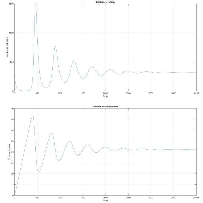
and  . In fact, numerical experiments with (3) and (6) show that the numbers of collisions
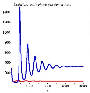
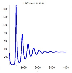

 , and the volume fraction multiplied by
  (due to the very large difference in magnitude between
  ,
,  ,
,  and
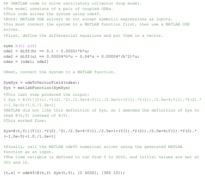
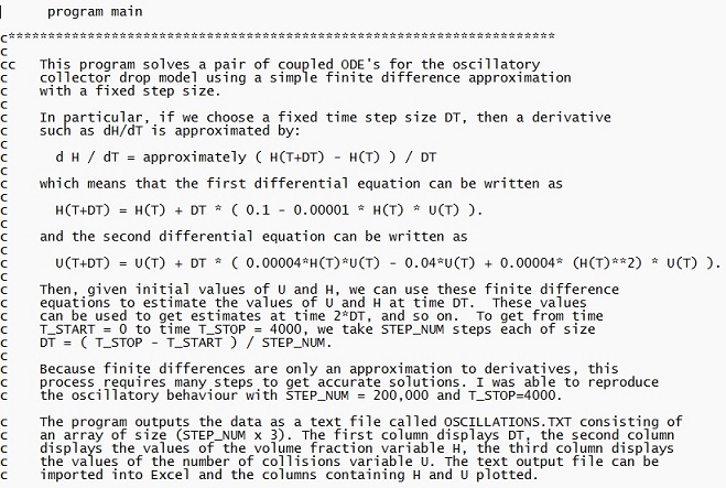
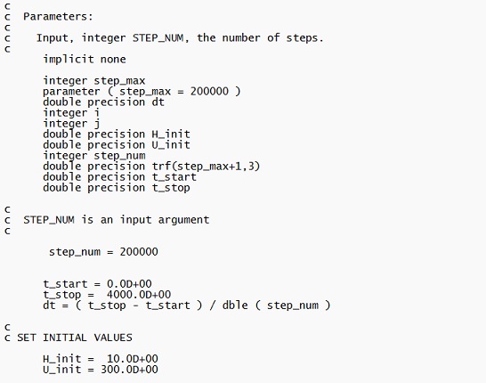
and  . (As a check, identical results were obtained using MATLAB and FORTRAN. See the screenshots below).
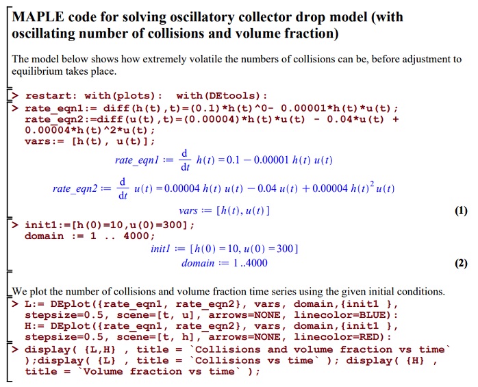


 be a set of
  and let
  be a continuous function defined on
  of degree
  or less which satisfies the interpolation conditions
 . This unique polynomial can be constructed by defining for
 except
  satisfy
 is Kronecker’s delta. In other words, for each
  , and
, and  for
for  . Lagrange’s polynomial interpolation formula is then written as
 in (4) causes all the terms to vanish except
  , so (1) is obtained. Crucially for the proofs below, the formula (4) represents a
  at the interpolation points
  respectively.
 . In the style of (4), this formula would be
 in (6) is unique. Therefore we can immediately conclude that
  . But (5) is simply
  , so it is immediately proved.
 . The left-hand side of (7) looks like Lagrange’s formula for interpolating the points
  . In the style of (4), this formula would be
 in (8) is a polynomial of degree
  , and the interpolating polynomial
  . But (7) is then simply
  , so it is immediately proved.
![f(\bar{T}_1) = \big[\mathcal{N}_1!\big]^{\gamma - 1}(\bar{T}_1)^{\mathcal{N}_1} + \big[(\mathcal{N} - \mathcal{N}_1)!\big]^{- 1}\bigg(\frac{\mathcal{N}!}{\mathcal{N}_1!}\bigg)^{\gamma}(\bar{T} - \bar{T}_1)^{\mathcal{N}-\mathcal{N}_1}](https://s0.wp.com/latex.php?latex=f%28%5Cbar%7BT%7D_1%29+%3D+%5Cbig%5B%5Cmathcal%7BN%7D_1%21%5Cbig%5D%5E%7B%5Cgamma+-+1%7D%28%5Cbar%7BT%7D_1%29%5E%7B%5Cmathcal%7BN%7D_1%7D+%2B+%5Cbig%5B%28%5Cmathcal%7BN%7D+-+%5Cmathcal%7BN%7D_1%29%21%5Cbig%5D%5E%7B-+1%7D%5Cbigg%28%5Cfrac%7B%5Cmathcal%7BN%7D%21%7D%7B%5Cmathcal%7BN%7D_1%21%7D%5Cbigg%29%5E%7B%5Cgamma%7D%28%5Cbar%7BT%7D+-+%5Cbar%7BT%7D_1%29%5E%7B%5Cmathcal%7BN%7D-%5Cmathcal%7BN%7D_1%7D&bg=ffffff&fg=111111&s=0&c=20201002)
 , ideally obtaining a closed form solution for the critical value
  . The precise context is not relevant here – I just want to record an asymptotic approximation trick I was able to use to solve this problem. Differentiating and setting equal to zero we obtain the first-order condition
![\mathcal{N}_1 \big[\mathcal{N}_1!\big]^{\gamma - 1}(\bar{T}_1^{\ast})^{\mathcal{N}_1-1}](https://s0.wp.com/latex.php?latex=%5Cmathcal%7BN%7D_1+%5Cbig%5B%5Cmathcal%7BN%7D_1%21%5Cbig%5D%5E%7B%5Cgamma+-+1%7D%28%5Cbar%7BT%7D_1%5E%7B%5Cast%7D%29%5E%7B%5Cmathcal%7BN%7D_1-1%7D&bg=ffffff&fg=111111&s=0&c=20201002)
![- (\mathcal{N} - \mathcal{N}_1)\big[(\mathcal{N} - \mathcal{N}_1)!\big]^{- 1}\bigg(\frac{\mathcal{N}!}{\mathcal{N}_1!}\bigg)^{\gamma}(\bar{T} - \bar{T}_1^{\ast})^{\mathcal{N}-\mathcal{N}_1 - 1} = 0](https://s0.wp.com/latex.php?latex=-+%28%5Cmathcal%7BN%7D+-+%5Cmathcal%7BN%7D_1%29%5Cbig%5B%28%5Cmathcal%7BN%7D+-+%5Cmathcal%7BN%7D_1%29%21%5Cbig%5D%5E%7B-+1%7D%5Cbigg%28%5Cfrac%7B%5Cmathcal%7BN%7D%21%7D%7B%5Cmathcal%7BN%7D_1%21%7D%5Cbigg%29%5E%7B%5Cgamma%7D%28%5Cbar%7BT%7D+-+%5Cbar%7BT%7D_1%5E%7B%5Cast%7D%29%5E%7B%5Cmathcal%7BN%7D-%5Cmathcal%7BN%7D_1+-+1%7D+%3D+0&bg=ffffff&fg=111111&s=0&c=20201002)
![\frac{(\bar{T}_1^{\ast})^{\mathcal{N}_1-1}}{(\bar{T} - \bar{T}_1^{\ast})^{\mathcal{N}-\mathcal{N}_1 - 1}} = \frac{(\mathcal{N} - \mathcal{N}_1)\big[(\mathcal{N} - \mathcal{N}_1)!\big]^{- 1}\bigg(\frac{\mathcal{N}!}{\mathcal{N}_1!}\bigg)^{\gamma}}{\mathcal{N}_1 \big[\mathcal{N}_1!\big]^{\gamma - 1}} = \frac{\big[\mathcal{N}!\big]^{\gamma}(\mathcal{N}_1-1)!}{\big[\mathcal{N}_1!\big]^{2\gamma}(\mathcal{N}-\mathcal{N}_1-1)!} \qquad \qquad \qquad (1)](https://s0.wp.com/latex.php?latex=%5Cfrac%7B%28%5Cbar%7BT%7D_1%5E%7B%5Cast%7D%29%5E%7B%5Cmathcal%7BN%7D_1-1%7D%7D%7B%28%5Cbar%7BT%7D+-+%5Cbar%7BT%7D_1%5E%7B%5Cast%7D%29%5E%7B%5Cmathcal%7BN%7D-%5Cmathcal%7BN%7D_1+-+1%7D%7D+%3D+%5Cfrac%7B%28%5Cmathcal%7BN%7D+-+%5Cmathcal%7BN%7D_1%29%5Cbig%5B%28%5Cmathcal%7BN%7D+-+%5Cmathcal%7BN%7D_1%29%21%5Cbig%5D%5E%7B-+1%7D%5Cbigg%28%5Cfrac%7B%5Cmathcal%7BN%7D%21%7D%7B%5Cmathcal%7BN%7D_1%21%7D%5Cbigg%29%5E%7B%5Cgamma%7D%7D%7B%5Cmathcal%7BN%7D_1+%5Cbig%5B%5Cmathcal%7BN%7D_1%21%5Cbig%5D%5E%7B%5Cgamma+-+1%7D%7D+%3D+%5Cfrac%7B%5Cbig%5B%5Cmathcal%7BN%7D%21%5Cbig%5D%5E%7B%5Cgamma%7D%28%5Cmathcal%7BN%7D_1-1%29%21%7D%7B%5Cbig%5B%5Cmathcal%7BN%7D_1%21%5Cbig%5D%5E%7B2%5Cgamma%7D%28%5Cmathcal%7BN%7D-%5Cmathcal%7BN%7D_1-1%29%21%7D+%5Cqquad+%5Cqquad+%5Cqquad+%281%29&bg=ffffff&fg=111111&s=0&c=20201002)
 , and
, and  , we can in fact satisfactorily approximate the left-hand side as


 as
as![(\mathcal{N}-\mathcal{N}_1) \cdot \frac{(\bar{T}_1^{\ast})^{\mathcal{N}_1}}{\bar{T}^{\mathcal{N}-\mathcal{N}_1}} = \frac{[\Gamma(\mathcal{N}+1)]^{\gamma}\cdot [\Gamma(\mathcal{N}_1)]}{[\Gamma(\mathcal{N}_1+1)]^{2\gamma} \cdot [\Gamma(\mathcal{N}-\mathcal{N}_1)]}](https://s0.wp.com/latex.php?latex=%28%5Cmathcal%7BN%7D-%5Cmathcal%7BN%7D_1%29+%5Ccdot+%5Cfrac%7B%28%5Cbar%7BT%7D_1%5E%7B%5Cast%7D%29%5E%7B%5Cmathcal%7BN%7D_1%7D%7D%7B%5Cbar%7BT%7D%5E%7B%5Cmathcal%7BN%7D-%5Cmathcal%7BN%7D_1%7D%7D+%3D+%5Cfrac%7B%5B%5CGamma%28%5Cmathcal%7BN%7D%2B1%29%5D%5E%7B%5Cgamma%7D%5Ccdot+%5B%5CGamma%28%5Cmathcal%7BN%7D_1%29%5D%7D%7B%5B%5CGamma%28%5Cmathcal%7BN%7D_1%2B1%29%5D%5E%7B2%5Cgamma%7D+%5Ccdot+%5B%5CGamma%28%5Cmathcal%7BN%7D-%5Cmathcal%7BN%7D_1%29%5D%7D&bg=ffffff&fg=111111&s=0&c=20201002)
![T_1^{\ast} = \frac{ [\Gamma(\mathcal{N}+1)]^{\frac{\gamma}{\mathcal{N}_1}} \cdot [\Gamma(\mathcal{N}_1)]^{\frac{1}{\mathcal{N}_1}} \cdot \bar{T}^{\ \frac{(\mathcal{N}-\mathcal{N}_1)}{\mathcal{N}_1}}}{(\mathcal{N} - \mathcal{N}_1)^{\frac{1}{\mathcal{N}_1}}\cdot [\Gamma(\mathcal{N}_1+1)]^{\frac{2\gamma}{\mathcal{N}_1}}\cdot [\Gamma(\mathcal{N}-\mathcal{N}_1)]^{\frac{1}{\mathcal{N}_1}}}](https://s0.wp.com/latex.php?latex=T_1%5E%7B%5Cast%7D+%3D+%5Cfrac%7B+%5B%5CGamma%28%5Cmathcal%7BN%7D%2B1%29%5D%5E%7B%5Cfrac%7B%5Cgamma%7D%7B%5Cmathcal%7BN%7D_1%7D%7D+%5Ccdot+%5B%5CGamma%28%5Cmathcal%7BN%7D_1%29%5D%5E%7B%5Cfrac%7B1%7D%7B%5Cmathcal%7BN%7D_1%7D%7D+%5Ccdot+%5Cbar%7BT%7D%5E%7B%5C+%5Cfrac%7B%28%5Cmathcal%7BN%7D-%5Cmathcal%7BN%7D_1%29%7D%7B%5Cmathcal%7BN%7D_1%7D%7D%7D%7B%28%5Cmathcal%7BN%7D+-+%5Cmathcal%7BN%7D_1%29%5E%7B%5Cfrac%7B1%7D%7B%5Cmathcal%7BN%7D_1%7D%7D%5Ccdot+%5B%5CGamma%28%5Cmathcal%7BN%7D_1%2B1%29%5D%5E%7B%5Cfrac%7B2%5Cgamma%7D%7B%5Cmathcal%7BN%7D_1%7D%7D%5Ccdot+%5B%5CGamma%28%5Cmathcal%7BN%7D-%5Cmathcal%7BN%7D_1%29%5D%5E%7B%5Cfrac%7B1%7D%7B%5Cmathcal%7BN%7D_1%7D%7D%7D&bg=ffffff&fg=111111&s=0&c=20201002)
 with probability density function
 . The cumulant generating function is the log-Laplace transform of
  , obtained as

 for the integral to converge in this case.

 ? One thing to notice is that this result is immediately obtainable from standard tables of Laplace transforms. For example, in most such tables one will find something like

 ,
,  and
and  in (5), we can then immediately deduce from (5) that

 . The basic procedure is simple. First, we convert
  , so the function
  in (8) is then
 , where
  and
and  are polynomials such that the degree of
 has a pole of order 1 at
  , so there is a single residue which can be obtained as
 as per (1) above, which in the notation of (9) translates into the condition
  . So, picking an arbitrary
  , we have the following:
 is designed to enclose the singularity of the integrand in the contour integral

 , the integral along the arc vanishes, and so

 and also


 on the arc, with
  , we must have
  since we are operating in the second and third quadrants, so


![\phi_X(t) = E[e^{itX}]](https://s0.wp.com/latex.php?latex=%5Cphi_X%28t%29+%3D+E%5Be%5E%7BitX%7D%5D&bg=ffffff&fg=111111&s=0&c=20201002) of an exponential random variate
of an exponential random variate 
 and thereby recover the density

![= \bigg[-\frac{1}{(\lambda - it)} e^{-(\lambda - it)x}\bigg]_0^{\infty}](https://s0.wp.com/latex.php?latex=%3D+%5Cbigg%5B-%5Cfrac%7B1%7D%7B%28%5Clambda+-+it%29%7D+e%5E%7B-%28%5Clambda+-+it%29x%7D%5Cbigg%5D_0%5E%7B%5Cinfty%7D&bg=ffffff&fg=111111&s=0&c=20201002)


 as
as  if
if  ).
).

 to
to  ). It quickly transpires that elementary techniques will not work easily with (5), so we try contour integration using the residue theorem. We turn the integration variable
  , and formulate the integral in (5) as a contour integral
 . To find the residue of the integrand at this pole, we multiply the integrand by
  , obtaining
  , and then evaluate this result at
  , yielding
  . Thus,
  , then Cauchy’s residue theorem tells us that the integral in (6) equals
  times the residue
 be some initial starting value, we can try the following:

 . First, noting that
  is half the circumference of a circle of radius
  , we have


![= \ln \bigg(\frac{1}{\mu} \bigg[ -\frac{\mu}{1-\mu k}e^{-(1-\mu k)x/\mu} \bigg]_0^{\infty} \bigg)](https://s0.wp.com/latex.php?latex=%3D+%5Cln+%5Cbigg%28%5Cfrac%7B1%7D%7B%5Cmu%7D+%5Cbigg%5B+-%5Cfrac%7B%5Cmu%7D%7B1-%5Cmu+k%7De%5E%7B-%281-%5Cmu+k%29x%2F%5Cmu%7D+%5Cbigg%5D_0%5E%7B%5Cinfty%7D+%5Cbigg%29&bg=ffffff&fg=111111&s=0&c=20201002)


 and that the natural logarithm is defined only if the Laplace transform parameter
  . Since


 , and the logarithm in (3) is now only defined for values of
  . What interested me is that it is not only the admissible region of values of
