A mathematics and physics `scrapbook', with notes on miscellaneous things that catch my interest in a range of areas including: mathematical methods; number theory; probability theory; stochastic processes; mathematical economics; econometrics; quantum theory; relativity theory; cosmology; cloud physics; statistical mechanics; nonlinear dynamics; electronic engineering; graph and network theory; mathematics in Latin; computational mathematics using Python and other maths software.
Markov’s inequality is a basic tool for putting upper bounds on tail probabilities. To derive it, suppose is a non-negative random variable. We want to put an upper bound on the tail probability where . We do this by observing that
where is the indicator function which takes the value 1 when and the value 0 otherwise. (It is obvious that (1) above holds, simply by the definition of this indicator function). Taking expectations of both sides of (1) we get
But
(by the law of total probability), so we can write
and so
This is Markov’s inequality. It can be modified, and thereby made sharper for particular situations, by considering a non-decreasing and non-negative function defined on an interval containing the values of . Then we have
As an example of applying this modified version, note that we obtain Chebyshev’s inequality by using the function , and defining . Putting these in (3) we get
More generally, we can get a version of Markov’s inequality involving the Laplace transform of the random variable by specifying , where is a positive number. In this case, noting that since is monotonically increasing, Markov’s inequality implies
So, now the Laplace transform of appears in the upper bound.
The so-called Cramér-Chernoff bounding method determines the best possible bound for a tail probability that one can possibly obtain by using Markov’s inequality with an exponential function . (This is one of the ways to understand intuitively how the entropy function in large deviation theory arises – see below). To explain this, begin by writing (4) above as
Since this inequality holds for all , one may choose to minimise the upper bound in (5). Define the log of the Laplace transform as
for all . Then we can write (5) as
Since we are free to replace the right-hand side of (7) by its minimum, we can do so, and we thus obtain Chernoff’s inequality
where the right-hand side of
is known as the Cramér transform of (6). A straightforward argument, given in the Appendix below, shows that we can extend the supremum in (9) over all in the definition of the Cramér transform:
The expression on the right-hand side of (10) is known as the Fenchel-Legendre dual function of , and is exactly the Fenchel-Legendre transform that is used in large deviation theory. As discussed in the Appendix below, the Fenchel-Legendre transform will coincide with the Cramér transform at every , but will equal zero for .
If is differentiable, the Cramér transform can be computed by differentiating with respect to . The optimising value of is found by setting the derivative with respect to equal to zero, that is
where is such that
The strict convexity of implies that has an increasing inverse , so
This formula can be used to compute the Cramér transform explicitly in simple cases. As an example, consider an exponential variate with probability density
Then the log of the Laplace transform of the random variable is
Therefore
and so
Appendix
The Cramér transform on the right-hand side of (9) is a non-negative function because it is identically zero for all when (since ), so the supremum can always be chosen to be at least zero. Since the exponential function is convex, Jensen’s inequality applies to it, and we can write
Therefore
Applying this to our case, with , we get
Therefore, we will have for all negative values of that
whenever (because (17) will then hold a fortiori). But we are still free to choose the supremum on the right-hand side of (9) to be at least zero when , so we can formally extend the supremum on the right-hand side of (9) over all in the definition of the Cramér transform, thereby obtaining the Fenchel-Legendre transform in (10). Therefore, as stated in the main text, the Fenchel-Legendre transform will coincide with the Cramér transform at every .
To see that the Fenchel-Legendre transform is zero for whenever , observe that this inequality implies , but by Jensen’s inequality we will then have , so . Since the supremum can always be chosen to be at least zero, the Fenchel-Legendre transform will indeed always be set to zero in this case.
In relation to a calculation involving sums of random variables, I needed to differentiate with respect to a double integral of the form
The parameter appears in both upper limits, but appears on its own in the outer upper limit, and as in the inner upper limit. I went through the motions of using Liebniz’s Rule and was interested to see how it worked in this case. I have not seen anything like this anywhere else online, so I want to record it here.
Liebniz’s Rule in the case of a single integral works thus:
Here, is the antiderivative of . The trick in the double integral case is to treat the inner integral like the function in the single integral case above. So, we differentiate the outer integral treating the inner integral as the function in the single integral case, then we differentiate the inner integral in the normal way. Thus, we write
The first integral in the penultimate step vanishes because the upper limit is converted from into in the application of Liebniz’s Rule.
The state of a quantum mechanical system is described by an element , called a ket, from a Hilbert space, i.e., a vector space that is complete and equipped with an inner product as well as a norm related to this inner product. Using bra-ket notation, the inner product of vectors and is represented as . In quantum mechanics, this inner product is not necessarily a real number, and we have the rule .
An observable is represented by a hermitian operator, say . A general operator acting on a ket gives another ket, . The inner product rule is then , where is the hermitian conjugate of . However, a hermitian operator has the inner product rule , and therefore . This is the defining property of a hermitian operator, and it is straightforward to show that satisfaction of this inner product rule implies the eigenvalues of must be real.
For an observable represented by the hermitian operator , we can always find an orthonormal basis of the state space that consists of the eigenvectors of . In the discrete spectrum case, for example, the eigenvectors of might be and the corresponding eigenvalues . (The discussion can easily be adapted to the continuous spectrum case by replacing summation by integration, and sequences of discrete coefficients by continuous functions, etc.) In order to perform the measurement of the observable on the quantum state , we would first need to expand the state using as basis vectors the eigenvectors of . We can do this using a projection operator
Thus the expansion of in terms of the eigenvectors of would be given by
where the expansion coefficient is the projection of on the axis represented by the i-th eigenvector of . (Notice that the quantum state itself remains unchanged by the action of projection operators like . Only the representation of changes, with respect to the eigenvectors of different hermitian operators).
Given the expansion of the ket
we then have a corresponding expansion of the bra, given by
The quantum state is normalised so that
where the absence of cross-products of the eigenvectors of , and the penultimate equality in (5), follow from the orthonormality of the eigenvectors of . Thus, the sequence of squares of the absolute values of the expansion coefficients, , can be regarded as representing a probability distribution.
We can use this probability distribution to calculate the expected value of the measurement of the observable :
In the case of two non-commuting hermitian operators, and , we can easily derive Heisenberg’s uncertainty principle using this mathematical structure, as follows. Let
and
be the expectations of and , computed as per (6). Let
be corresponding deviations from the mean. (Note that and must be hermitian if and are, since they are obtained simply by subtracting a real number). Then the mean squared deviations are
And by the Cauchy-Schwarz inequality, we can write
Therefore we have
(Notice that we introduced the norm brackets in (13) to allow for the fact that will in general be a complex number. The expression is not hermitian, even though and are).
Finally, observe that
Using this in (14) gives us the key inequality of the Heisenberg uncertainty principle:
For example, in the case of the momentum and position operators in one dimension, we have
Putting (17) into (16) then gives the canonical inequality of the Heisenberg uncertainty principle:
We consider a free particle restricted to a ring of length , with a complete lap around the ring taken to begin at position and end at position . The general TISE is
where
We take in the ring and we assume the periodic boundary condition .
The TISE becomes
which has general solution
In principle, this allows for two independent solutions superposed with coefficients and . However, the periodic boundary condition implies which in turn implies , and periodic boundary conditions produce travelling waves, not standing waves. Therefore, the presence of both terms in the general solution above is a superposition of two running waves with the same amplitude but travelling in opposite directions. One of these running waves is superfluous for the purposes of developing the solution below, so we can set and just focus on the forward travelling wave. The general solution then reduces to
The periodic boundary condition requires to be an integer multiple of , so using where and are the -th energy and momentum states respectively (and note that this expression for as is allowed only because in the ring), we have
and
Choosing units equivalent to setting , we can write the -th wave function as
To find the normalising constant , we write
so . The solutions for the particle in a ring are then travelling waves of the form
with corresponding momentum and energy states
and
respectively.
Note that the solutions here are travelling waves, and are different from the standing wave solutions obtained for the more commonly encountered particle-in-a-box problem with left- and right-hand endpoints and respectively, and with non-periodic boundary conditions . When no boundary conditions are specified at all, i.e., the particle is not confined to a box or a ring, then with the TISE and its general solution are the same as those initially obtained above, but energy and momentum are no longer quantized, i.e., they can take any values along a continuum.
A mass connected to a spring and executing simple harmonic motion will oscillate at a natural frequency which is independent of the initial position or velocity of the mass. The particular pattern of vibration at the natural frequency is referred to as the mode of vibration corresponding to that natural frequency. Obviously, there is only one natural frequency and one corresponding mode of vibration for a single mass on a spring. However, a system consisting of two coupled masses connected by springs will, in general, have two distinct natural frequencies (the natural frequencies are often referred to as harmonic frequencies, or simply as harmonics), and two distinct modes of vibration corresponding to these natural frequencies. In general, a system consisting of masses connected by springs will have natural frequencies and a distinct mode of vibration for each of these natural frequencies.
With this in mind, it is interesting to observe that the displacements from equilibrium of an oscillating system of masses connected to springs can be described BOTH in terms of a coupled system of ODEs, AND as an uncoupled system of ODEs, with each independent ODE in the uncoupled system representing a distinct mode of vibration of the original system characterised by a distinct natural frequency. A specific example of this will be given shortly. Amazingly, the same kind of idea also applies to the Hamiltonian of a vibrating lattice of quantum oscillators. The Hamiltonian will initially be expressed in a complicated way involving coupling of the quantum oscillators. However, with some strategic Fourier transforms, the Hamiltonian will be re-expressed in terms of uncoupled entities, each entity representing a distinct mode of vibration of the original lattice characterised by a distinct natural frequency. The transformed Hamiltonian will look exactly the same as the Hamiltonian for an uncoupled set of quantum harmonic oscillators, and quasiparticles called phonons will emerge in this framework as discrete packets of vibrational energy. These phonons are closely analogous to photons as carriers of discrete packets of energy in the context of electromagnetism.
Before considering the case of quantum oscillators in a lattice, it is instructive to explore a specific example of the situation for ODEs describing a simple mass-spring system. Consider two identical pendulums, and , connected by a spring whose relaxed length is exactly equal to the distance between the pendulum bobs.
Suppose the system is displaced from equilibrium by moving the pendulums away from their relaxed positions and releasing them. The second picture above shows an arbitrary moment when the displacement of pendulum is and the displacement of pendulum is . Since the spring is being stretched by an amount , the magnitude of the restoring force on is
(i.e., the usual gravitational restoring force for a pendulum, plus the restoring force due to the spring). For , the magnitude of the restoring force is
(the gravitational and spring restoring forces are opposing each other, as can be seen in the sketch above). Therefore using the usual equations and for a spring system, the equations of motion for and are
Dividing through by , and letting , we can write these as
These are a pair of coupled ODEs, but we can easily manipulate equations (1) and (2) to obtain two independent ODEs from them. Adding the two equations gives
and subtracting (2) from (1) gives
Writing and , we can re-express these as
These are now two uncoupled ODEs for simple harmonic oscillations, the first one having natural frequency and the second one having natural frequency . They are independent oscillations because, according to equations (3) and (4), changes in occur independently of changes in , and vice versa. They can be solved independently to get sinusoidal expressions for and . For example, and are possible solutions. The transformed equations (3) and (4) represent another way of describing the two normal modes of vibration occurring in the original coupled system (1) and (2), one normal mode having frequency , the other having the higher frequency .
The present note is concerned with a similar idea at the quantum level, where we imagine quantum oscillators connected linearly by forces which act like little springs, i.e., a 1-D lattice of quantum oscillators. We want to transform the Hamiltonian for this coupled system into a Hamiltonian which looks like the Hamiltonian for a system of independent quantum harmonic oscillators. Analogous to the transformed ODE system for the two-mass system considered above, the transformed Hamiltonian will be expressed in terms of the possible modes of vibration of the original coupled system. The vibration energies in this reformulated Hamiltonian will be seen to consist of discrete `packets’ of energy, , which can be added to, or subtracted from, particular quantum oscillators in the lattice using creation and annihilation operators, just as in the usual quantum harmonic oscillator framework. As stated earlier, these discrete packets of energy can be regarded as particles (or, rather, quasiparticles) analogous to photons in electromagnetism, and they are referred to as phonons in the solid state physics literature. A phonon is thus a quantum of vibrational energy, , needed to move a lattice of coupled quantum oscillators up or down to different vibrational energy levels.
So, we consider a one-dimensional chain of connected quantum particles, each of mass , connected by forces which act like springs of unstretched length and with spring constant .
The -th mass is normally at position , but can be displaced slightly by amount . Writing the quantum mechanical momentum and position operators as and respectively, the Hamiltonian operator for the system (a generalisation of the Hamiltonian for a collection of uncoupled quantum oscillators) is
Although this system consists of masses which are strongly coupled to their neighbours by springs, we will show that if the system is perturbed from an initial state where each mass is at position (e.g., by stretching and releasing some of the springs), the vibrations of the 1-D lattice behave as if the system consisted of a set of uncoupled quantum harmonic oscillators. In other words, the Hamiltonian in (5) can be re-expressed in the form
where is Planck’s constant, is a natural frequency of the system depending on , and and are creation and annihilation operators respectively (as in the context of the quantum harmonic oscillator). The subscript on the creation and annihilation operators reflects the fact that they are only able to act on the -th oscillator in the system, having no effect on the others. Thus, each oscillator in the system is understood to have its own pair of creation and annihilation operators.
We begin by applying discrete Fourier transforms to the position and momentum operators and appearing in (5):
We impose periodic boundary conditions, so that
Therefore, we must have
so
where can take integer values between and inclusive, i.e., is in the set of least positive residues of .
An important observation is that
because when we have a sum of terms on the left-hand side each equal to , whereas when we can use the formula for the sum of a geometric progression to write
since . The result in (14) is used repeatedly in what follows.
Note that (8) is the inverse transform for (7), and (10) is the inverse transform for (9). To see how this works, let us confirm that using (8) in the right-hand side of (7) gives . Making the substitution we get
(using (14))
as claimed, since the only non-zero term in the sum in the penultimate line is the one corresponding to . Thus, in (8) is the inverse operator of in (7), and likewise in (10) is the inverse operator of in (9).
Next, we observe that for the usual operators in (7) and (9) we have the commutation relations
The inverse transforms in (8) and (10) then imply that we have the following commutation relations for the inverse operators:
To see this, observe that we have
(using (15))
(using (14))
as claimed.
With these results we are now in a position to work out the terms in the Hamiltonian in (5) above in terms of the inverse operators and . First, using (9), we have
(carrying out the spatial sum)
(using (14))
where in the last step we used the Kronecker delta to carry out one of the momentum sums. This has the effect of setting (because any term not satisfying this will disappear), leaving us with a sum over a single index.
Next, using (7), we have
Subtracting (7) from this we get
Using this to deal with the other terms in the Hamiltonian in (5) we get
(using the result ).
Using (17) and (18), we can rewrite the Hamiltonian in (5) as
where .
Next, we observe from (10) that the Hermitian conjugate of is given by
But since is Hermitian, we have . Therefore
A similar argument using (8) shows that
[Formally, the adjoint of an operator is defined by . In the case of a Hermitian operator, we have . Therefore, . This guarantees that the operator has real eigenvalues. In our case, by working out the inner products and , for example, we would find that they are equal, confirming that ].
Using these results with (16), we can write down the commutation relation between and as
We can also write down the creation and annihilation operators (cf. the quantum harmonic oscillator) as
It is easy to show that these satisfy the commutation relations
Therefore, creation and annihilation operators with subscript can only act on an oscillator corresponding to the same wave vector . When they try to act on an oscillator corresponding to a different wave vector, they commute, so they are unable to have any effect. To demonstrate (27) in the case , we have
as required.
We can invert equations (23) and (24). From (24) we get
so
Using (28) to substitute for in (23) we get, with some easy manipulations,
And using (29) to substitute for in (28) we get
Therefore, using (29), we deduce
and, similarly, using (30) we deduce
Adding (31) and (32) we get
Therefore the Hamiltonian in (19) becomes
But, by inspection, and are the same operators, just expressed with different indices. Therefore, re-indexing this term in the Hamiltonian in (34) we get
Finally, using the commutator in (27) with , we have
Therefore, the Hamiltonian in (35) can be written as
which is the same as (6). This result shows that the Hamiltonian for a linear chain of coupled quantum oscillators can be expressed in terms of modes of vibration which behave like independent and uncoupled quantum harmonic oscillators. The -th mode of vibration can accept increments to its energy in integer multiples of a basic quantum of energy, . As in the standard quantum harmonic oscillator model, these quanta of energy behave like particles, and we call these quanta phonons in the present context.
I was struggling to explain the concept of a solid angle to a student. I found that the following approach, by analogy with plane angles, succeeded.
In the case of a plane angle (in radians) subtended by an arc length , the following relationship holds:
On the left-hand side we have the ratio of to the circumference of a unit circle, . On the right-hand side, we have the ratio of the arc length to the circumference of a circle of radius , . So, the idea is that is a measure of the part of the circumference of the unit circle at the apex that is covered by the projection of on to this unit circle. From (1) we get
(or the familiar formula for calculating arc lengths, ).
A solid angle is simply a 3D analogue of this.
Instead of a unit circle at the apex, we have a unit sphere with surface area . The solid angle (in steradians) is subtended by the area element , and these satisfy the following relationship:
On the left-hand side we have the ratio of to the surface area of the unit sphere, . On the right-hand side, we have the ratio of the area element to the surface area of a sphere of radius , . So, the idea is that is a measure of the part of the surface area of the unit sphere at the apex that is covered by the projection of on to this unit sphere. From (3), we get the familiar formula for solid angles,
It is possible to solve some simple problems involving solid angles purely by symmetry considerations. For example, to work out the solid angle subtended by one of the faces of a cube, we note that the cube has six faces of equal area and together they must account for the entire surface area of the unit sphere at the apex. Therefore, a single cube face must account for one-sixth of the surface area of the unit sphere at the apex, so we have
Therefore, a single cube face subtends a solid angle of steradians.
A Laplace transform of a function is defined by the equation
The idea is that a Laplace transform takes as an input a function of , , and yields as the output a function of , .
In many applications of this idea, for example when applying a Laplace transform to the solution of a differential equation, we need to find the inverse of the transform to obtain the required solution. This can often be done by consulting tables of Laplace transforms and their inverses in reference manuals, but we can also invert Laplace transforms using something called the Bromwich integral. I want to explore the latter approach in this note, as it involves the useful trick of solving integrals by converting them to contour integration problems on the complex plane. I also want to record a useful trick for changing the order of integration in double integrals which is employed in the proof of a convolution theorem for Laplace transforms.
Differential equations can be solved using Laplace transforms by finding the transforms of derivatives , , etc. To find , we use the above definition of and integrate by parts as follows:
where for simplicity we have written and .
To find , we think of as and substitute for in (2) to get
Continuing this process, we can also obtain the transforms of higher derivatives. Using these results, we can now solve differential equations. For example, suppose we want to solve
with initial conditions and . We simply take the Laplace transform of each term in the equation. We get
Using the given initial conditions, the left-hand side of (5) reduces to . We can obtain the Laplace transform on the right-hand side of (5) by consulting a reference table, or by integrating. Following the latter approach, we integrate by parts once to get
and then integrate by parts again to get
Combining these, we get
Alternatively, from standard reference tables we find that
Therefore
Using these results in (5) we get
and so
Recall that , so what we need to do now to solve the problem is to apply an inverse Laplace transform to both sides of (7). This would give
We could evaluate the right-hand side of (8) using the formula from the reference table in (6). We see from this formula that we need , , so we can immediately conclude that
This is the required solution to the second-order differential equation in (4) above. What I want to do now is explore the Bromwich integral for Laplace transforms, and use it to confirm the answer in (9) by obtaining the inverse Laplace transform of via the residue theorem from complex analysis.
In the definition of the Laplace transform in (1) above, we now let be a complex number, say . Then the Laplace transform becomes
where for some real . [We must have some restriction on to make the integral converge at infinity. The restriction depends on what the function is, but it is always of the form for some real . To illustrate this idea, consider the case . Then we have
The final equality here holds only for , because otherwise would not vanish at the upper limit of the integral. If is complex, then would be required in this case]. Now, (10) has a form similar to that of a Fourier transform
with inverse
in (10) corresponds to in (11), and in (11) corresponds to in (10). Pursuing this analogy with a Fourier transform, the inverse transform for (10), corresponding to (12), would then be
Using the definition of , we can write this as
for . Since is a constant in this setup, we have , so we can write (14) as
where the notation means that we integrate along a vertical line in the plane. [This can be any vertical line on which as required by the restriction on ]. The integral (15) for the inverse Laplace transform is called the Bromwich integral.
To use (15) to evaluate for a given , we exploit the fact that we can evaluate integrals in the complex plane by using the residue theorem. We imagine a contour consisting of a vertical straight line and a semicircle enclosing an area to the left of . We evaluate (15) by using this contour.
We restrict to be of the form , with and polynomials, and of degree at least one higher than . The value of the integral around the contour is determined by the singularities lying inside the semicircle, in accordance with the residue theorem. Specifically, the residue theorem says that the integral around the contour equals times the sum of the residues of at its poles. As the radius of the semicircle goes to infinity, the integral along the straight line becomes an improper integral from to . However, the integral around the semicircle has the radius appearing to a higher degree in the denominator than in the numerator, so this integral goes to zero as the radius becomes infinite. We are left only with the improper integral along the straight line, and the residue theorem then assures us that this must equal times the sum of the residues of at its poles . Cancelling the factor from (15), we conclude that
So, to find from the Laplace transform , we simply construct the complex function , and then sum the residues at all the poles of this constructed function. Note that we must include all poles in (16), i.e., we must choose such that all the poles of lie inside the contour to the left of the vertical line we are integrating along. To find the residues at each pole, we can use the following rule:
When a function has a pole of order at , the residue at this pole can be obtained by multiplying by , differentiating the result times, dividing by , and evaluating the resulting expression at .
We can now apply this approach to find the inverse of the transform
We have
This has a pole of order 5 at . Therefore, multiplying by we get , differentiating this result times we get , and dividing by we get . Finally, evaluating the result at gives the answer
which exactly matches the answer we got in (9) above.
We also have a convolution theorem for Laplace transforms, the proof of which I want to explore here. The convolution theorem says that the Laplace transform of a convolution of functions is the product of the Laplace transforms of the individual functions in the convolution. So, if and are functions, and and are their corresponding Laplace transforms, then the convolution theorem says
where
is the convolution of and . To prove (17), note that from the definition of a Laplace transform in (1) above we have
We will now rewrite this by replacing by different dummy variables of integration so that we can write the product of the two integrals as a double integral. We then have
We now make the change of variables in the inner integral in (19), i.e., the integral with respect to , so that is treated as fixed. Then , , and when we have , while when we have . Then (19) becomes
We will now change the order of integration using the following diagrams to interpret what is going on in (20):
From the first diagram, we see that the double integral in (20) is over the area to the right of the diagonal line. Within a given strip of width , the integral adds up little area elements from the line to , then the integral sums over the horizontal strips from to , covering the whole infinite area to the right of the diagonal line. However, we can obtain exactly the same result by considering a vertical strip of width as shown in the second diagram. Changing the order of integration and integrating with respect to first, then within the given strip of width , the integral adds up little area elements from to the line , and then the integral sums over the vertical strips from to . In doing things this way round, we are working with the double integral
where the last step follows from the definition of a Laplace transform in (1) above. As per the construction in the diagrams, the two integrals (20) and (21) must be the same, so the convolution theorem in (17) is proved. The proof is useful in showing how a double infinite integral can be converted into a double integral in which only one of the integrals is improper, and vice versa. I have come across the need for this technique in different contexts.
In this note, I want to quickly record a couple of interesting results involving the beta function. First, consider the reciprocal beta function
where
It is easy to see by using Stirling’s formula
in the numerator and denominator of that
for with fixed. Therefore, the reciprocal beta function converges to a simple power law.
Second, we can easily show that the beta function converges when summed over by exchanging the summation and integration operations. We obtain the infinite sum of the beta function as
I sometimes see things like or instead of the usual . Where do these strange notations come from? Suppose we have a random variable , considered as a function which maps events from a -field to an interval on the real line. Let the random variable take values in the range , which we will partition into subintervals , with , , , , and with , . The random variable maps each event in the -field to a corresponding interval on the real line according to a probability distribution. Pick an arbitrary point in each subinterval . Form a simple random variable from by assigning to each the value . Then the expectation of is given by
But if we denote the probability distribution function of by , we have
Therefore we can write
Therefore the notation means: the weighted sum of the t values, where the weights are the probabilities given by the difference in the values of the probability distribution function at the endpoints of the interval corresponding to t. But the approximations improve as the subdivisions become finer, so we can suppose to be given by
So the notation means: the weighted sum of the t values, where the weights are the probabilities given by the difference in the values of the probability distribution function at the endpoints of the differential interval .
In the case of absolutely continuous random variables, we have a density function , so
where denotes the -th interval length for over which can be regarded as being approximately constant. This implies
As the subdivisions become finer, both of the above approximations improve. On the basis of this informal argument, we should then have
Therefore we have two equivalent notations in the absolutely continuous case:
Suppose we divide a time interval of length into steps. Let be a random variable with initial value . At the first step, the value of the random variable can go up by or down by with probability and respectively. (This is a Bernoulli trial with probability of success ). Then at the first step we have and the expected value and variance are
and
At the second step we similarly have with the same expected value and variance. And so on. This step-by-step process is a discrete-time random walk. Now let
be the position after steps. Then is a binomial random variable with expected value
and variance
We now want to pass to continuous time by letting or equivalently , and we want to make the expected value and variance independent of and in this limit. For this purpose, we need to define
where and are two parameters whose role will become clear shortly. Substituting these three into the expressions for and and passing to the limit we get the expected value
and variance
Thus, in the limit as , both the mean and variance are independent of and . Note in particular that must depend on the square root of for this to be achieved. Were it not for this, the mean and variance would depend on and on the number of steps .
Now, as the number of steps becomes large, the binomial random variable becomes normally distributed, with
Let . Then we have
or
Passing to differentials we then have the stochastic differential equation of Brownian motion with drift:
where
is the (infinitesimal) increment of a Wiener process (also known as Brownian motion), is a drift parameter, and is a variance parameter. Note that in the increment of the Wiener process we have and is serially uncorrelated, i.e., for . Thus, the values of for any two different time intervals are independent, so follows a Markov process with independent increments. We have and . Therefore the variance of the change in a Wiener process grows linearly with the time horizon.
Note that the Wiener process does not have a time derivative in the conventional sense because with
we have
and this becomes infinite when we try to pass to the limit . This is why we need to use Itô calculus to deal with Brownian motion and related processes, rather than being able to use conventional calculus.
Brownian motion with drift is a simple generalisation of the Wiener process. Over any time interval , the change in , , is normally distributed with and . From the above development starting with a discrete-time random walk, we can now see why must depend on the square root of , not just on .


![t \cdot P(Y \geq t) \leq E[Y \cdot 1_{\{Y \geq t\}}]](https://s0.wp.com/latex.php?latex=t+%5Ccdot+P%28Y+%5Cgeq+t%29+%5Cleq+E%5BY+%5Ccdot+1_%7B%5C%7BY+%5Cgeq+t%5C%7D%7D%5D&bg=ffffff&fg=111111&s=0&c=20201002)
![E[Y \cdot 1_{\{Y \geq t\}}] = E[Y | Y \geq t] P(Y \geq t)](https://s0.wp.com/latex.php?latex=E%5BY+%5Ccdot+1_%7B%5C%7BY+%5Cgeq+t%5C%7D%7D%5D+%3D+E%5BY+%7C+Y+%5Cgeq+t%5D+P%28Y+%5Cgeq+t%29&bg=ffffff&fg=111111&s=0&c=20201002)
![\leq E[Y | Y \geq t] P(Y \geq t) + E[Y | Y < t] P(Y < t)](https://s0.wp.com/latex.php?latex=%5Cleq+E%5BY+%7C+Y+%5Cgeq+t%5D+P%28Y+%5Cgeq+t%29+%2B+E%5BY+%7C+Y+%3C+t%5D+P%28Y+%3C+t%29&bg=ffffff&fg=111111&s=0&c=20201002)
![= E[Y]](https://s0.wp.com/latex.php?latex=%3D+E%5BY%5D&bg=ffffff&fg=111111&s=0&c=20201002)
![t \cdot P(Y \geq t) \leq E[Y]](https://s0.wp.com/latex.php?latex=t+%5Ccdot+P%28Y+%5Cgeq+t%29+%5Cleq+E%5BY%5D&bg=ffffff&fg=111111&s=0&c=20201002)
![P(Y \geq t) \leq \frac{E[Y]}{t} \qquad \qquad \qquad (2)](https://s0.wp.com/latex.php?latex=P%28Y+%5Cgeq+t%29+%5Cleq+%5Cfrac%7BE%5BY%5D%7D%7Bt%7D+%5Cqquad+%5Cqquad+%5Cqquad+%282%29&bg=ffffff&fg=111111&s=0&c=20201002)

![P(\phi(Y) \geq \phi(t)) \leq \frac{E[\phi(Y)]}{\phi(t)} \qquad \qquad \qquad (3)](https://s0.wp.com/latex.php?latex=P%28%5Cphi%28Y%29+%5Cgeq+%5Cphi%28t%29%29+%5Cleq+%5Cfrac%7BE%5B%5Cphi%28Y%29%5D%7D%7B%5Cphi%28t%29%7D+%5Cqquad+%5Cqquad+%5Cqquad+%283%29&bg=ffffff&fg=111111&s=0&c=20201002)

![Y = Z - E[Z]](https://s0.wp.com/latex.php?latex=Y+%3D+Z+-+E%5BZ%5D&bg=ffffff&fg=111111&s=0&c=20201002)
![P(|Z - E[Z]| \geq t) \leq \frac{Var[Z]}{t^2}](https://s0.wp.com/latex.php?latex=P%28%7CZ+-+E%5BZ%5D%7C+%5Cgeq+t%29+%5Cleq+%5Cfrac%7BVar%5BZ%5D%7D%7Bt%5E2%7D&bg=ffffff&fg=111111&s=0&c=20201002)


![P(Z \geq t) \leq \frac{E[e^{kZ}]}{e^{kt}} \qquad \qquad \qquad (4)](https://s0.wp.com/latex.php?latex=P%28Z+%5Cgeq+t%29+%5Cleq+%5Cfrac%7BE%5Be%5E%7BkZ%7D%5D%7D%7Be%5E%7Bkt%7D%7D+%5Cqquad+%5Cqquad+%5Cqquad+%284%29&bg=ffffff&fg=111111&s=0&c=20201002)
![P(Z \geq t) \leq e^{-kt} E[e^{kZ}] \qquad \qquad \qquad (5)](https://s0.wp.com/latex.php?latex=P%28Z+%5Cgeq+t%29+%5Cleq+e%5E%7B-kt%7D+E%5Be%5E%7BkZ%7D%5D+%5Cqquad+%5Cqquad+%5Cqquad+%285%29&bg=ffffff&fg=111111&s=0&c=20201002)

![\lambda(k) = \ln E[e^{kz}] \qquad \qquad \qquad (6)](https://s0.wp.com/latex.php?latex=%5Clambda%28k%29+%3D+%5Cln+E%5Be%5E%7Bkz%7D%5D+%5Cqquad+%5Cqquad+%5Cqquad+%286%29&bg=ffffff&fg=111111&s=0&c=20201002)


![t \geq E[Z]](https://s0.wp.com/latex.php?latex=t+%5Cgeq+E%5BZ%5D&bg=ffffff&fg=111111&s=0&c=20201002)
![t < E[Z]](https://s0.wp.com/latex.php?latex=t+%3C+E%5BZ%5D&bg=ffffff&fg=111111&s=0&c=20201002)


![\lambda(k) = \ln E[e^{kX}] = -\ln(1 + \mu k) \qquad \qquad \qquad (15)](https://s0.wp.com/latex.php?latex=%5Clambda%28k%29+%3D+%5Cln+E%5Be%5E%7BkX%7D%5D+%3D+-%5Cln%281+%2B+%5Cmu+k%29+%5Cqquad+%5Cqquad+%5Cqquad+%2815%29&bg=ffffff&fg=111111&s=0&c=20201002)


![e^{E[X]} \leq E[e^{X}]](https://s0.wp.com/latex.php?latex=e%5E%7BE%5BX%5D%7D+%5Cleq+E%5Be%5E%7BX%7D%5D&bg=ffffff&fg=111111&s=0&c=20201002)
![\ln E[e^X] \geq E[X]](https://s0.wp.com/latex.php?latex=%5Cln+E%5Be%5EX%5D+%5Cgeq+E%5BX%5D&bg=ffffff&fg=111111&s=0&c=20201002)

![\lambda(k) \geq k E[Z] \qquad \qquad \qquad (17)](https://s0.wp.com/latex.php?latex=%5Clambda%28k%29+%5Cgeq+k+E%5BZ%5D+%5Cqquad+%5Cqquad+%5Cqquad+%2817%29&bg=ffffff&fg=111111&s=0&c=20201002)


![kt < kE[Z]](https://s0.wp.com/latex.php?latex=kt+%3C+kE%5BZ%5D&bg=ffffff&fg=111111&s=0&c=20201002)
![\lambda(k) \geq kE[Z] > kt](https://s0.wp.com/latex.php?latex=%5Clambda%28k%29+%5Cgeq+kE%5BZ%5D+%3E+kt&bg=ffffff&fg=111111&s=0&c=20201002)

 a double integral of the form
 in the inner upper limit. I went through the motions of using Liebniz’s Rule and was interested to see how it worked in this case. I have not seen anything like this anywhere else online, so I want to record it here.
 ![\frac{d}{dx} \int_0^x f(t) dt = \frac{d}{dx} \big[F(x) - F(0)\big] = f(x)](https://s0.wp.com/latex.php?latex=%5Cfrac%7Bd%7D%7Bdx%7D+%5Cint_0%5Ex+f%28t%29+dt+%3D+%5Cfrac%7Bd%7D%7Bdx%7D+%5Cbig%5BF%28x%29+-+F%280%29%5Cbig%5D+%3D+f%28x%29&bg=ffffff&fg=111111&s=0&c=20201002)
 is the antiderivative of
  . The trick in the double integral case is to treat the inner integral like the function in the single integral case above. So, we differentiate the outer integral treating the inner integral as the function in the single integral case, then we differentiate the inner integral in the normal way. Thus, we write


 in the application of Liebniz’s Rule.
  , called a ket, from a Hilbert space, i.e., a vector space that is complete and equipped with an inner product as well as a norm related to this inner product. Using bra-ket notation, the inner product of vectors
  and
and  . In quantum mechanics, this inner product is not necessarily a real number, and we have the rule
  .
.  . A general operator
  acting on a ket
  . The inner product rule is then
  , where
  is the hermitian conjugate of
  , and therefore
  . This is the defining property of a hermitian operator, and it is straightforward to show that satisfaction of this inner product rule implies the eigenvalues of
  and the corresponding eigenvalues
  . (The discussion can easily be adapted to the continuous spectrum case by replacing summation by integration, and sequences of discrete coefficients by continuous functions, etc.) In order to perform the measurement of the observable on the quantum state

 is the projection of
  . Only the representation of


 , can be regarded as representing a probability distribution.


 , we can easily derive Heisenberg’s uncertainty principle using this mathematical structure, as follows. Let


 and
and  must be hermitian if
  and
and  are, since they are obtained simply by subtracting a real number). Then the mean squared deviations are


![= \frac{1}{4} |\langle [\hat{Q}^{\prime}, \hat{R}^{\prime}] \rangle|^2 \qquad \qquad \qquad (13)](https://s0.wp.com/latex.php?latex=%3D+%5Cfrac%7B1%7D%7B4%7D+%7C%5Clangle+%5B%5Chat%7BQ%7D%5E%7B%5Cprime%7D%2C+%5Chat%7BR%7D%5E%7B%5Cprime%7D%5D+%5Crangle%7C%5E2+%5Cqquad+%5Cqquad+%5Cqquad+%2813%29&bg=ffffff&fg=111111&s=0&c=20201002)
![\Delta q \Delta r \ge \frac{1}{2} |\langle [\hat{Q}^{\prime}, \hat{R}^{\prime}] \rangle| \qquad \qquad \qquad (14)](https://s0.wp.com/latex.php?latex=%5CDelta+q+%5CDelta+r+%5Cge+%5Cfrac%7B1%7D%7B2%7D+%7C%5Clangle+%5B%5Chat%7BQ%7D%5E%7B%5Cprime%7D%2C+%5Chat%7BR%7D%5E%7B%5Cprime%7D%5D+%5Crangle%7C+%5Cqquad+%5Cqquad+%5Cqquad+%2814%29&bg=ffffff&fg=111111&s=0&c=20201002)
 will in general be a complex number. The expression
  is not hermitian, even though
 ![[\hat{Q}^{\prime}, \hat{R}^{\prime}] = \hat{Q}^{\prime}\hat{R}^{\prime} - \hat{R}^{\prime} \hat{Q}^{\prime} = [\hat{Q}, \hat{R}] \qquad \qquad \qquad (15)](https://s0.wp.com/latex.php?latex=%5B%5Chat%7BQ%7D%5E%7B%5Cprime%7D%2C+%5Chat%7BR%7D%5E%7B%5Cprime%7D%5D+%3D+%5Chat%7BQ%7D%5E%7B%5Cprime%7D%5Chat%7BR%7D%5E%7B%5Cprime%7D+-+%5Chat%7BR%7D%5E%7B%5Cprime%7D+%5Chat%7BQ%7D%5E%7B%5Cprime%7D+%3D+%5B%5Chat%7BQ%7D%2C+%5Chat%7BR%7D%5D+%5Cqquad+%5Cqquad+%5Cqquad+%2815%29&bg=ffffff&fg=111111&s=0&c=20201002)
![\Delta q \Delta r \ge \frac{1}{2} |\langle [\hat{Q}, \hat{R}] \rangle| \qquad \qquad \qquad (16)](https://s0.wp.com/latex.php?latex=%5CDelta+q+%5CDelta+r+%5Cge+%5Cfrac%7B1%7D%7B2%7D+%7C%5Clangle+%5B%5Chat%7BQ%7D%2C+%5Chat%7BR%7D%5D+%5Crangle%7C+%5Cqquad+%5Cqquad+%5Cqquad+%2816%29&bg=ffffff&fg=111111&s=0&c=20201002)
![[\hat{P}, \hat{X}] = -i \hbar \qquad \qquad \qquad (17)](https://s0.wp.com/latex.php?latex=%5B%5Chat%7BP%7D%2C+%5Chat%7BX%7D%5D+%3D+-i+%5Chbar+%5Cqquad+%5Cqquad+%5Cqquad+%2817%29&bg=ffffff&fg=111111&s=0&c=20201002)

 , with a complete lap around the ring taken to begin at position
  and end at position
  . The general TISE is
 ![\big[\frac{\hat{p}^2}{2m} + V(x)\big]\psi = E\psi](https://s0.wp.com/latex.php?latex=%5Cbig%5B%5Cfrac%7B%5Chat%7Bp%7D%5E2%7D%7B2m%7D+%2B+V%28x%29%5Cbig%5D%5Cpsi+%3D+E%5Cpsi&bg=ffffff&fg=111111&s=0&c=20201002)

 in the ring and we assume the periodic boundary condition
  .
.

 and
and  . However, the periodic boundary condition implies
  which in turn implies
  , and periodic boundary conditions produce travelling waves, not standing waves. Therefore, the presence of both terms in the general solution above is a superposition of two running waves with the same amplitude but travelling in opposite directions. One of these running waves is superfluous for the purposes of developing the solution below, so we can set
  and just focus on the forward travelling wave. The general solution then reduces to
 to be an integer multiple of
  , so using
  where
where  and
and  are the
  -th energy and momentum states respectively (and note that this expression for
  is allowed only because

 , we can write the

 . The solutions for the particle in a ring are then travelling waves of the form


 and
and  . When no boundary conditions are specified at all, i.e., the particle is not confined to a box or a ring, then with
  masses connected by springs will have
  is exactly equal to the distance between the pendulum bobs.
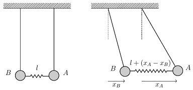
 and the displacement of pendulum
  . Since the spring is being stretched by an amount
  , the magnitude of the restoring force on

 and
and  for a spring system, the equations of motion for

 , and letting
  , we can write these as


 and
and  , we can re-express these as

 and the second one having natural frequency
  . They are independent oscillations because, according to equations (3) and (4), changes in
  occur independently of changes in
  , and vice versa. They can be solved independently to get sinusoidal expressions for
  and
and  are possible solutions. The transformed equations (3) and (4) represent another way of describing the two normal modes of vibration occurring in the original coupled system (1) and (2), one normal mode having frequency
  , which can be added to, or subtracted from, particular quantum oscillators in the lattice using creation and annihilation operators, just as in the usual quantum harmonic oscillator framework. As stated earlier, these discrete packets of energy can be regarded as particles (or, rather, quasiparticles) analogous to photons in electromagnetism, and they are referred to as phonons in the solid state physics literature. A phonon is thus a quantum of vibrational energy,
  and with spring constant
  .
. 
 -th mass is normally at position
  , but can be displaced slightly by amount
  . Writing the quantum mechanical momentum and position operators as
  and
and  respectively, the Hamiltonian operator for the system (a generalisation of the Hamiltonian for a collection of uncoupled quantum oscillators) is
 ![\hat{H} = \sum_{j=0}^{N-1} \bigg[\frac{\hat{p}_j^{2}}{2m} + \frac{1}{2}K(\hat{x}_{j+1}-\hat{x}_j)^2 \bigg] \qquad \qquad \qquad (5)](https://s0.wp.com/latex.php?latex=%5Chat%7BH%7D+%3D+%5Csum_%7Bj%3D0%7D%5E%7BN-1%7D+%5Cbigg%5B%5Cfrac%7B%5Chat%7Bp%7D_j%5E%7B2%7D%7D%7B2m%7D+%2B+%5Cfrac%7B1%7D%7B2%7DK%28%5Chat%7Bx%7D_%7Bj%2B1%7D-%5Chat%7Bx%7D_j%29%5E2+%5Cbigg%5D+%5Cqquad+%5Cqquad+%5Cqquad+%285%29&bg=ffffff&fg=111111&s=0&c=20201002)

 is Planck’s constant,
  is a natural frequency of the system depending on
  and
and  are creation and annihilation operators respectively (as in the context of the quantum harmonic oscillator). The subscript
  appearing in (5):


 inclusive, i.e.,
 , whereas when
  we can use the formula for the sum of a geometric progression to write
 . The result in (14) is used repeatedly in what follows.
 ![\frac{1}{\sqrt{N}} \sum_{k=0}^{N-1} \bigg[\frac{1}{\sqrt{N}}\sum_{j^{\prime}=0}^{N-1}\hat{x}_{j^{\prime}} e^{- i k j^{\prime} a}\bigg] e^{i k j a}](https://s0.wp.com/latex.php?latex=%5Cfrac%7B1%7D%7B%5Csqrt%7BN%7D%7D+%5Csum_%7Bk%3D0%7D%5E%7BN-1%7D+%5Cbigg%5B%5Cfrac%7B1%7D%7B%5Csqrt%7BN%7D%7D%5Csum_%7Bj%5E%7B%5Cprime%7D%3D0%7D%5E%7BN-1%7D%5Chat%7Bx%7D_%7Bj%5E%7B%5Cprime%7D%7D+e%5E%7B-+i+k+j%5E%7B%5Cprime%7D+a%7D%5Cbigg%5D+e%5E%7Bi+k+j+a%7D&bg=ffffff&fg=111111&s=0&c=20201002)
![= \frac{1}{N} \sum_{j^{\prime}=0}^{N-1} \hat{x}_j^{\prime} \bigg[\sum_{k=0}^{N-1} e^{- i k (j^{\prime}-j)a}\bigg]](https://s0.wp.com/latex.php?latex=%3D+%5Cfrac%7B1%7D%7BN%7D+%5Csum_%7Bj%5E%7B%5Cprime%7D%3D0%7D%5E%7BN-1%7D+%5Chat%7Bx%7D_j%5E%7B%5Cprime%7D+%5Cbigg%5B%5Csum_%7Bk%3D0%7D%5E%7BN-1%7D+e%5E%7B-+i+k+%28j%5E%7B%5Cprime%7D-j%29a%7D%5Cbigg%5D&bg=ffffff&fg=111111&s=0&c=20201002)


 . Thus,
  in (8) is the inverse operator of
  in (10) is the inverse operator of
 ![[\hat{x}_j, \hat{p}_{j^{\prime}}] = i \hbar \delta_{j, j^{\prime}} \qquad \qquad \qquad (15)](https://s0.wp.com/latex.php?latex=%5B%5Chat%7Bx%7D_j%2C+%5Chat%7Bp%7D_%7Bj%5E%7B%5Cprime%7D%7D%5D+%3D+i+%5Chbar+%5Cdelta_%7Bj%2C+j%5E%7B%5Cprime%7D%7D+%5Cqquad+%5Cqquad+%5Cqquad+%2815%29&bg=ffffff&fg=111111&s=0&c=20201002)
![[\hat{x}_k, \hat{p}_{k^{\prime}}] = i \hbar \delta_{k, -k^{\prime}} \qquad \qquad \qquad (16)](https://s0.wp.com/latex.php?latex=%5B%5Chat%7Bx%7D_k%2C+%5Chat%7Bp%7D_%7Bk%5E%7B%5Cprime%7D%7D%5D+%3D+i+%5Chbar+%5Cdelta_%7Bk%2C+-k%5E%7B%5Cprime%7D%7D+%5Cqquad+%5Cqquad+%5Cqquad+%2816%29&bg=ffffff&fg=111111&s=0&c=20201002)
![[\hat{x}_k, \hat{p}_{k^{\prime}}] = \frac{1}{\sqrt{N}} \sum_{j=0}^{N-1} \hat{x}_j e^{- i k j a} \cdot \frac{1}{\sqrt{N}} \sum_{j^{\prime}=0}^{N-1} \hat{p}_{j^{\prime}} e^{-i k^{\prime} j^{\prime} a}](https://s0.wp.com/latex.php?latex=%5B%5Chat%7Bx%7D_k%2C+%5Chat%7Bp%7D_%7Bk%5E%7B%5Cprime%7D%7D%5D+%3D+%5Cfrac%7B1%7D%7B%5Csqrt%7BN%7D%7D+%5Csum_%7Bj%3D0%7D%5E%7BN-1%7D+%5Chat%7Bx%7D_j+e%5E%7B-+i+k+j+a%7D+%5Ccdot+%5Cfrac%7B1%7D%7B%5Csqrt%7BN%7D%7D+%5Csum_%7Bj%5E%7B%5Cprime%7D%3D0%7D%5E%7BN-1%7D+%5Chat%7Bp%7D_%7Bj%5E%7B%5Cprime%7D%7D+e%5E%7B-i+k%5E%7B%5Cprime%7D+j%5E%7B%5Cprime%7D+a%7D&bg=ffffff&fg=111111&s=0&c=20201002)

![= \frac{1}{N} \sum_{j=0}^{N-1} \sum_{j^{\prime}=0}^{N-1} e^{-i k j a} e^{- i k^{\prime} j^{\prime} a} [\hat{x}_j, \hat{p}_{j^{\prime}}]](https://s0.wp.com/latex.php?latex=%3D+%5Cfrac%7B1%7D%7BN%7D+%5Csum_%7Bj%3D0%7D%5E%7BN-1%7D++%5Csum_%7Bj%5E%7B%5Cprime%7D%3D0%7D%5E%7BN-1%7D+e%5E%7B-i+k+j+a%7D+e%5E%7B-+i+k%5E%7B%5Cprime%7D+j%5E%7B%5Cprime%7D+a%7D++%5B%5Chat%7Bx%7D_j%2C+%5Chat%7Bp%7D_%7Bj%5E%7B%5Cprime%7D%7D%5D&bg=ffffff&fg=111111&s=0&c=20201002)


 (because any term not satisfying this will disappear), leaving us with a sum over a single index.


 ).
). ![\hat{H} = \sum_{k=0}^{N-1} \bigg[\frac{1}{2m} \hat{p}_k \hat{p}_{-k} + \frac{1}{2} m \omega_k^2 \hat{x}_k \hat{x}_{-k} \bigg] \qquad \qquad \qquad (19)](https://s0.wp.com/latex.php?latex=%5Chat%7BH%7D+%3D+%5Csum_%7Bk%3D0%7D%5E%7BN-1%7D+%5Cbigg%5B%5Cfrac%7B1%7D%7B2m%7D+%5Chat%7Bp%7D_k+%5Chat%7Bp%7D_%7B-k%7D+%2B+%5Cfrac%7B1%7D%7B2%7D+m+%5Comega_k%5E2+%5Chat%7Bx%7D_k+%5Chat%7Bx%7D_%7B-k%7D+%5Cbigg%5D+%5Cqquad+%5Cqquad+%5Cqquad+%2819%29&bg=ffffff&fg=111111&s=0&c=20201002)
 .
. 
 . Therefore

 . In the case of a Hermitian operator, we have
  . Therefore,
  . This guarantees that the operator has real eigenvalues. In our case, by working out the inner products
  and
and  , for example, we would find that they are equal, confirming that
  as
as ![[\hat{x}_k, \hat{p}_{k^{\prime}}^{\dag}] = [\hat{x}_k, \hat{p}_{-k^{\prime}}] = i \hbar \delta_{k, k^{\prime}} \qquad \qquad \qquad (22)](https://s0.wp.com/latex.php?latex=%5B%5Chat%7Bx%7D_k%2C+%5Chat%7Bp%7D_%7Bk%5E%7B%5Cprime%7D%7D%5E%7B%5Cdag%7D%5D+%3D+%5B%5Chat%7Bx%7D_k%2C+%5Chat%7Bp%7D_%7B-k%5E%7B%5Cprime%7D%7D%5D+%3D+i+%5Chbar+%5Cdelta_%7Bk%2C+k%5E%7B%5Cprime%7D%7D+%5Cqquad+%5Cqquad+%5Cqquad+%2822%29&bg=ffffff&fg=111111&s=0&c=20201002)


![[\hat{a}_k^{\dag}, \hat{a}_{k^{\prime}}^{\dag}] = 0 \qquad \qquad \qquad \ \ \ (25)](https://s0.wp.com/latex.php?latex=%5B%5Chat%7Ba%7D_k%5E%7B%5Cdag%7D%2C+%5Chat%7Ba%7D_%7Bk%5E%7B%5Cprime%7D%7D%5E%7B%5Cdag%7D%5D+%3D+0+%5Cqquad+%5Cqquad+%5Cqquad+%5C++%5C++%5C+%2825%29&bg=ffffff&fg=111111&s=0&c=20201002)
![[\hat{a}_k, \hat{a}_{k^{\prime}}] = 0 \qquad \qquad \qquad \ \ \ (26)](https://s0.wp.com/latex.php?latex=%5B%5Chat%7Ba%7D_k%2C+%5Chat%7Ba%7D_%7Bk%5E%7B%5Cprime%7D%7D%5D+%3D+0+%5Cqquad+%5Cqquad+%5Cqquad+%5C++%5C++%5C+%2826%29&bg=ffffff&fg=111111&s=0&c=20201002)
![[\hat{a}_k, \hat{a}_{k^{\prime}}^{\dag}] = \delta_{k, k^{\prime}} \qquad \qquad \qquad (27)](https://s0.wp.com/latex.php?latex=%5B%5Chat%7Ba%7D_k%2C+%5Chat%7Ba%7D_%7Bk%5E%7B%5Cprime%7D%7D%5E%7B%5Cdag%7D%5D+%3D+%5Cdelta_%7Bk%2C+k%5E%7B%5Cprime%7D%7D+%5Cqquad+%5Cqquad+%5Cqquad+%2827%29&bg=ffffff&fg=111111&s=0&c=20201002)
 , we have
![[\hat{a}_k, \hat{a}_k^{\dag}] = \hat{a}_k \hat{a}_k^{\dag} - \hat{a}_k^{\dag} \hat{a}_k](https://s0.wp.com/latex.php?latex=%5B%5Chat%7Ba%7D_k%2C+%5Chat%7Ba%7D_k%5E%7B%5Cdag%7D%5D+%3D+%5Chat%7Ba%7D_k+%5Chat%7Ba%7D_k%5E%7B%5Cdag%7D+-++%5Chat%7Ba%7D_k%5E%7B%5Cdag%7D++%5Chat%7Ba%7D_k&bg=ffffff&fg=111111&s=0&c=20201002)
![= \frac{m \omega_k}{2 \hbar} \bigg[\big(\hat{x}_k + \frac{i}{m \omega_k} \hat{p}_k\big) \big(\hat{x}_{-k} - \frac{i}{m \omega_k} \hat{p}_{-k}\big) - \big(\hat{x}_{-k} - \frac{i}{m \omega_k} \hat{p}_{-k}\big) \big(\hat{x}_k + \frac{i}{m \omega_k} \hat{p}_k\big)\bigg]](https://s0.wp.com/latex.php?latex=%3D+%5Cfrac%7Bm+%5Comega_k%7D%7B2+%5Chbar%7D+%5Cbigg%5B%5Cbig%28%5Chat%7Bx%7D_k+%2B+%5Cfrac%7Bi%7D%7Bm+%5Comega_k%7D+%5Chat%7Bp%7D_k%5Cbig%29+%5Cbig%28%5Chat%7Bx%7D_%7B-k%7D+-+%5Cfrac%7Bi%7D%7Bm+%5Comega_k%7D+%5Chat%7Bp%7D_%7B-k%7D%5Cbig%29+-++%5Cbig%28%5Chat%7Bx%7D_%7B-k%7D+-+%5Cfrac%7Bi%7D%7Bm+%5Comega_k%7D+%5Chat%7Bp%7D_%7B-k%7D%5Cbig%29+%5Cbig%28%5Chat%7Bx%7D_k+%2B+%5Cfrac%7Bi%7D%7Bm+%5Comega_k%7D+%5Chat%7Bp%7D_k%5Cbig%29%5Cbigg%5D&bg=ffffff&fg=111111&s=0&c=20201002)
![= \frac{m \omega_k}{2 \hbar} \bigg[-\frac{i}{m \omega_k}\hat{x}_k\hat{p}_{-k} + \frac{i}{m\omega_k}\hat{p}_k\hat{x}_{-k} - \frac{i}{m\omega_k}\hat{x}_{-k}\hat{p}_k + \frac{i}{m\omega_k}\hat{p}_{-k}\hat{x}_k\bigg]](https://s0.wp.com/latex.php?latex=%3D+%5Cfrac%7Bm+%5Comega_k%7D%7B2+%5Chbar%7D+%5Cbigg%5B-%5Cfrac%7Bi%7D%7Bm+%5Comega_k%7D%5Chat%7Bx%7D_k%5Chat%7Bp%7D_%7B-k%7D+%2B+%5Cfrac%7Bi%7D%7Bm%5Comega_k%7D%5Chat%7Bp%7D_k%5Chat%7Bx%7D_%7B-k%7D+-+%5Cfrac%7Bi%7D%7Bm%5Comega_k%7D%5Chat%7Bx%7D_%7B-k%7D%5Chat%7Bp%7D_k+%2B+%5Cfrac%7Bi%7D%7Bm%5Comega_k%7D%5Chat%7Bp%7D_%7B-k%7D%5Chat%7Bx%7D_k%5Cbigg%5D&bg=ffffff&fg=111111&s=0&c=20201002)
![= \frac{m \omega_k}{2 \hbar} \bigg[-\frac{i}{m\omega_k}[\hat{x}_k, \hat{p}_{-k}] + \frac{i}{m\omega_k}[\hat{p}_k, \hat{x}_{-k}]\bigg]](https://s0.wp.com/latex.php?latex=%3D+%5Cfrac%7Bm+%5Comega_k%7D%7B2+%5Chbar%7D+%5Cbigg%5B-%5Cfrac%7Bi%7D%7Bm%5Comega_k%7D%5B%5Chat%7Bx%7D_k%2C+%5Chat%7Bp%7D_%7B-k%7D%5D+%2B+%5Cfrac%7Bi%7D%7Bm%5Comega_k%7D%5B%5Chat%7Bp%7D_k%2C+%5Chat%7Bx%7D_%7B-k%7D%5D%5Cbigg%5D&bg=ffffff&fg=111111&s=0&c=20201002)
![= \frac{m \omega_k}{2 \hbar} \bigg[-\frac{i}{m\omega_k}(i \hbar) + \frac{i}{m\omega_k}(-i\hbar)\bigg]](https://s0.wp.com/latex.php?latex=%3D+%5Cfrac%7Bm+%5Comega_k%7D%7B2+%5Chbar%7D+%5Cbigg%5B-%5Cfrac%7Bi%7D%7Bm%5Comega_k%7D%28i+%5Chbar%29+%2B+%5Cfrac%7Bi%7D%7Bm%5Comega_k%7D%28-i%5Chbar%29%5Cbigg%5D&bg=ffffff&fg=111111&s=0&c=20201002)


![\hat{H} = \sum_{k=0}^{N-1} \bigg[\frac{\hbar \omega_k}{2} \big(\hat{a}_k\hat{a}_k^{\dag} + \hat{a}_{-k}^{\dag} \hat{a}_{-k}\big) \bigg] \qquad \qquad \qquad (34)](https://s0.wp.com/latex.php?latex=%5Chat%7BH%7D+%3D+%5Csum_%7Bk%3D0%7D%5E%7BN-1%7D+%5Cbigg%5B%5Cfrac%7B%5Chbar+%5Comega_k%7D%7B2%7D+%5Cbig%28%5Chat%7Ba%7D_k%5Chat%7Ba%7D_k%5E%7B%5Cdag%7D+%2B+%5Chat%7Ba%7D_%7B-k%7D%5E%7B%5Cdag%7D+%5Chat%7Ba%7D_%7B-k%7D%5Cbig%29+%5Cbigg%5D+%5Cqquad+%5Cqquad+%5Cqquad+%2834%29&bg=ffffff&fg=111111&s=0&c=20201002)
 and
and  are the same operators, just expressed with different indices. Therefore, re-indexing this term in the Hamiltonian in (34) we get
 ![\hat{H} = \sum_{k=0}^{N-1} \bigg[\frac{\hbar \omega_k}{2} \big(\hat{a}_k\hat{a}_k^{\dag} + \hat{a}_{k}^{\dag} \hat{a}_{k}\big) \bigg] \qquad \qquad \qquad (35)](https://s0.wp.com/latex.php?latex=%5Chat%7BH%7D+%3D+%5Csum_%7Bk%3D0%7D%5E%7BN-1%7D+%5Cbigg%5B%5Cfrac%7B%5Chbar+%5Comega_k%7D%7B2%7D+%5Cbig%28%5Chat%7Ba%7D_k%5Chat%7Ba%7D_k%5E%7B%5Cdag%7D+%2B+%5Chat%7Ba%7D_%7Bk%7D%5E%7B%5Cdag%7D+%5Chat%7Ba%7D_%7Bk%7D%5Cbig%29+%5Cbigg%5D+%5Cqquad+%5Cqquad+%5Cqquad+%2835%29&bg=ffffff&fg=111111&s=0&c=20201002)

![\hat{H} = \sum_{k=0}^{N-1} \bigg[\hbar \omega_k \bigg(\hat{a}_{k}^{\dag} \hat{a}_{k} + \frac{1}{2}\bigg) \bigg] \qquad \qquad \qquad (36)](https://s0.wp.com/latex.php?latex=%5Chat%7BH%7D+%3D+%5Csum_%7Bk%3D0%7D%5E%7BN-1%7D+%5Cbigg%5B%5Chbar+%5Comega_k+%5Cbigg%28%5Chat%7Ba%7D_%7Bk%7D%5E%7B%5Cdag%7D+%5Chat%7Ba%7D_%7Bk%7D+%2B+%5Cfrac%7B1%7D%7B2%7D%5Cbigg%29+%5Cbigg%5D+%5Cqquad+%5Cqquad+%5Cqquad+%2836%29&bg=ffffff&fg=111111&s=0&c=20201002)

 (in radians) subtended by an arc length
  , the following relationship holds:
 . On the right-hand side, we have the ratio of the arc length
  ,
,  . So, the idea is that
 ).
). 
 . The solid angle
  (in steradians) is subtended by the area element
  , and these satisfy the following relationship:
 . So, the idea is that


 steradians.
  of a function
  is defined by the equation
 ,
,  .
.  ,
,  , etc. To find
  , we use the above definition of
![= \big[e^{-pt} y(t) \big]_0^{\infty} + p\int_0^{\infty} e^{-pt}y(t)dt](https://s0.wp.com/latex.php?latex=%3D+%5Cbig%5Be%5E%7B-pt%7D+y%28t%29+%5Cbig%5D_0%5E%7B%5Cinfty%7D+%2B+p%5Cint_0%5E%7B%5Cinfty%7D+e%5E%7B-pt%7Dy%28t%29dt&bg=ffffff&fg=111111&s=0&c=20201002)

 and
and  .
.  , we think of
  as
as  and substitute
  for
for  in (2) to get


 and
and  . We simply take the Laplace transform of each term in the equation. We get
 . We can obtain the Laplace transform on the right-hand side of (5) by consulting a reference table, or by integrating. Following the latter approach, we integrate by parts once to get


 , so what we need to do now to solve the problem is to apply an inverse Laplace transform to both sides of (7). This would give
 ,
,  , so we can immediately conclude that
 via the residue theorem from complex analysis.
  . Then the Laplace transform becomes

 for some real
  to make the integral converge at infinity. The restriction depends on what the function
  for some real
  . Then we have
![\int_0^{\infty} e^{-pt} dt = \big[ -\frac{1}{p}e^{-pt}\big]_0^{\infty} = \frac{1}{p}](https://s0.wp.com/latex.php?latex=%5Cint_0%5E%7B%5Cinfty%7D+e%5E%7B-pt%7D+dt+%3D+%5Cbig%5B+-%5Cfrac%7B1%7D%7Bp%7De%5E%7B-pt%7D%5Cbig%5D_0%5E%7B%5Cinfty%7D+%3D+%5Cfrac%7B1%7D%7Bp%7D&bg=ffffff&fg=111111&s=0&c=20201002)
 , because otherwise
  would not vanish at the upper limit of the integral. If
  would be required in this case]. Now, (10) has a form similar to that of a Fourier transform

 in (11), and
  in (10). Pursuing this analogy with a Fourier transform, the inverse transform for (10), corresponding to (12), would then be
 , we can write this as

 is a constant in this setup, we have
  , so we can write (14) as

 plane. [This can be any vertical line on which
  as required by the restriction on
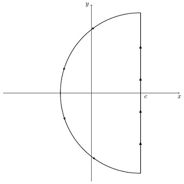
 to be of the form
  , with
  and
and  polynomials, and
  times the sum of the residues of
  at its poles. As the radius of the semicircle goes to infinity, the integral along the straight line becomes an improper integral from
  to
to  . However, the integral around the semicircle has the radius appearing to a higher degree in the denominator than in the numerator, so this integral goes to zero as the radius becomes infinite. We are left only with the improper integral along the straight line, and the residue theorem then assures us that this must equal
 has a pole of order
  , the residue at this pole can be obtained by multiplying
  , differentiating the result
  times, dividing by
  , and evaluating the resulting expression at
  .
. 

 . Therefore, multiplying by
  we get
  , differentiating this result
  times we get
  , and dividing by
  we get
  . Finally, evaluating the result at
 and
and  are functions, and
  and
and  are their corresponding Laplace transforms, then the convolution theorem says
![G(p)H(p) = L\bigg[\int_0^t g(t - \tau)h(\tau) d\tau \bigg] \qquad \qquad \qquad (17)](https://s0.wp.com/latex.php?latex=G%28p%29H%28p%29+%3D+L%5Cbigg%5B%5Cint_0%5Et+g%28t+-+%5Ctau%29h%28%5Ctau%29+d%5Ctau+%5Cbigg%5D+%5Cqquad+%5Cqquad+%5Cqquad+%2817%29&bg=ffffff&fg=111111&s=0&c=20201002)

 and
and  . To prove (17), note that from the definition of a Laplace transform in (1) above we have


 in the inner integral in (19), i.e., the integral with respect to
  , so that
  is treated as fixed. Then
  ,
,  , and when
  we have
  , while when
  we have
  . Then (19) becomes

 , the
, the  to
to  , covering the whole infinite area to the right of the diagonal line. However, we can obtain exactly the same result by considering a vertical strip of width
  as shown in the second diagram. Changing the order of integration and integrating with respect to
  , and then the
  to
to 
![= \int_{t=0}^{\infty} e^{-pt} \bigg[\int_{\tau=0}^t g(t-\tau)h(\tau) d\tau \bigg] dt](https://s0.wp.com/latex.php?latex=%3D+%5Cint_%7Bt%3D0%7D%5E%7B%5Cinfty%7D+e%5E%7B-pt%7D+%5Cbigg%5B%5Cint_%7B%5Ctau%3D0%7D%5Et++g%28t-%5Ctau%29h%28%5Ctau%29+d%5Ctau+%5Cbigg%5D+dt&bg=ffffff&fg=111111&s=0&c=20201002)
![= L\bigg[\int_0^t g(t-\tau)h(\tau) d\tau \bigg] \qquad \qquad \qquad (21)](https://s0.wp.com/latex.php?latex=%3D+L%5Cbigg%5B%5Cint_0%5Et++g%28t-%5Ctau%29h%28%5Ctau%29+d%5Ctau+%5Cbigg%5D+%5Cqquad+%5Cqquad+%5Cqquad+%2821%29&bg=ffffff&fg=111111&s=0&c=20201002)


 that
that
 with
with  fixed. Therefore, the reciprocal beta function

![E[X] = \int t dF_X(t)](https://s0.wp.com/latex.php?latex=E%5BX%5D+%3D+%5Cint+t+dF_X%28t%29&bg=ffffff&fg=111111&s=0&c=20201002) or
or ![E[X] = \int t F_X(dt)](https://s0.wp.com/latex.php?latex=E%5BX%5D+%3D+%5Cint+t+F_X%28dt%29&bg=ffffff&fg=111111&s=0&c=20201002) instead of the usual
instead of the usual ![E[X] = \int t f_X(t) dt](https://s0.wp.com/latex.php?latex=E%5BX%5D+%3D+%5Cint+t+f_X%28t%29+dt&bg=ffffff&fg=111111&s=0&c=20201002) . Where do these strange notations come from? Suppose we have a random variable
. Where do these strange notations come from? Suppose we have a random variable ![[a, b]](https://s0.wp.com/latex.php?latex=%5Ba%2C+b%5D&bg=ffffff&fg=111111&s=0&c=20201002) , which we will partition into
, which we will partition into  , with
  ,
,  ,
,  ,
, ![M_n \equiv [b_{n-1}, b_n]](https://s0.wp.com/latex.php?latex=M_n+%5Cequiv+%5Bb_%7Bn-1%7D%2C+b_n%5D&bg=ffffff&fg=111111&s=0&c=20201002) , and with
, and with  ,
,  . The random variable
  in the
  on the real line according to a probability distribution. Pick an arbitrary point
  in each subinterval
  from
from  . Then the expectation of
 ![E[X_s] = \sum_{i=1}^{n} t_i P(X_s = t_i) = \sum_{i=1}^{n} t_i P(X \in M_i)](https://s0.wp.com/latex.php?latex=E%5BX_s%5D+%3D+%5Csum_%7Bi%3D1%7D%5E%7Bn%7D+t_i+P%28X_s+%3D+t_i%29+%3D+%5Csum_%7Bi%3D1%7D%5E%7Bn%7D+t_i+P%28X+%5Cin+M_i%29&bg=ffffff&fg=111111&s=0&c=20201002)
 , we have
![E[X_s] = \sum_i t_i (F_X(b_i) - F_X(b_{i-1})) \approx \int t dF_X(t)](https://s0.wp.com/latex.php?latex=E%5BX_s%5D+%3D+%5Csum_i+t_i+%28F_X%28b_i%29+-+F_X%28b_%7Bi-1%7D%29%29+%5Capprox+%5Cint+t+dF_X%28t%29&bg=ffffff&fg=111111&s=0&c=20201002)
![E[X]](https://s0.wp.com/latex.php?latex=E%5BX%5D&bg=ffffff&fg=111111&s=0&c=20201002) to be given by
to be given by![E[X] = \int t dF_X(t) = \int t F_X(dt)](https://s0.wp.com/latex.php?latex=E%5BX%5D+%3D++%5Cint+t+dF_X%28t%29+%3D+%5Cint+t+F_X%28dt%29&bg=ffffff&fg=111111&s=0&c=20201002)
 means: the weighted sum of the t values, where the weights are the probabilities given by the difference in the values of the probability distribution function at the endpoints of the differential interval
  , so
, so 
 denotes the
  -th interval length for
 ![E[X_s] \approx \sum_i t_i f_X(t_i) \triangle_i t \approx \int t f_X(t) dt](https://s0.wp.com/latex.php?latex=E%5BX_s%5D+%5Capprox+%5Csum_i+t_i+f_X%28t_i%29+%5Ctriangle_i+t+%5Capprox+%5Cint+t+f_X%28t%29+dt&bg=ffffff&fg=111111&s=0&c=20201002)
![E[X] = \int t F_X(dt) = \int t f_X(t) dt](https://s0.wp.com/latex.php?latex=E%5BX%5D+%3D+%5Cint+t+F_X%28dt%29+%3D+%5Cint+t+f_X%28t%29+dt&bg=ffffff&fg=111111&s=0&c=20201002)
 into
into  steps. Let
  . At the first step, the value of the random variable can go up by
  or down by
  respectively. (This is a Bernoulli trial with probability of success
  and the expected value and variance are
![E[\Delta X_1] = p \Delta h - q \Delta h = (p - q) \Delta h](https://s0.wp.com/latex.php?latex=E%5B%5CDelta+X_1%5D+%3D+p+%5CDelta+h+-+q+%5CDelta+h+%3D+%28p+-+q%29+%5CDelta+h&bg=ffffff&fg=111111&s=0&c=20201002)
![V[\Delta X_1] = E[(\Delta X_1)^2] - E^2[\Delta X_1]](https://s0.wp.com/latex.php?latex=V%5B%5CDelta+X_1%5D+%3D+E%5B%28%5CDelta+X_1%29%5E2%5D+-+E%5E2%5B%5CDelta+X_1%5D&bg=ffffff&fg=111111&s=0&c=20201002)

![= (\Delta h)^2[p + q - (p - q)^2]](https://s0.wp.com/latex.php?latex=%3D+%28%5CDelta+h%29%5E2%5Bp+%2B+q+-+%28p+-+q%29%5E2%5D&bg=ffffff&fg=111111&s=0&c=20201002)

 with the same expected value and variance. And so on. This step-by-step process is a discrete-time random walk. Now let
 is a binomial random variable with expected value
![E[\Delta X_t] = E[\Delta X_1 + \Delta X_2 + \cdots + \Delta X_n] = n(p - q)\Delta h = \Delta t (p - q) \frac{\Delta h}{\Delta_n t}](https://s0.wp.com/latex.php?latex=E%5B%5CDelta+X_t%5D+%3D+E%5B%5CDelta+X_1+%2B+%5CDelta+X_2+%2B+%5Ccdots+%2B+%5CDelta+X_n%5D+%3D+n%28p+-+q%29%5CDelta+h+%3D+%5CDelta+t+%28p+-+q%29+%5Cfrac%7B%5CDelta+h%7D%7B%5CDelta_n+t%7D&bg=ffffff&fg=111111&s=0&c=20201002)
![V[\Delta X_t] = V[\Delta X_1 + \Delta X_2 + \cdots + \Delta X_n] = n4pq(\Delta h)^2 = 4pq\Delta t \frac{(\Delta h)^2}{\Delta_n t}](https://s0.wp.com/latex.php?latex=V%5B%5CDelta+X_t%5D+%3D+V%5B%5CDelta+X_1+%2B+%5CDelta+X_2+%2B+%5Ccdots+%2B+%5CDelta+X_n%5D+%3D+n4pq%28%5CDelta+h%29%5E2+%3D+4pq%5CDelta+t+%5Cfrac%7B%28%5CDelta+h%29%5E2%7D%7B%5CDelta_n+t%7D&bg=ffffff&fg=111111&s=0&c=20201002)
 or equivalently
  , and we want to make the expected value and variance independent of
  in this limit. For this purpose, we need to define
![p = \frac{1}{2} \bigg[1 + \frac{\alpha}{\sigma} \sqrt{\Delta_n t}\bigg]](https://s0.wp.com/latex.php?latex=p+%3D+%5Cfrac%7B1%7D%7B2%7D+%5Cbigg%5B1+%2B+%5Cfrac%7B%5Calpha%7D%7B%5Csigma%7D+%5Csqrt%7B%5CDelta_n+t%7D%5Cbigg%5D&bg=ffffff&fg=111111&s=0&c=20201002)
![q = \frac{1}{2} \bigg[1 - \frac{\alpha}{\sigma} \sqrt{\Delta_n t}\bigg]](https://s0.wp.com/latex.php?latex=q+%3D+%5Cfrac%7B1%7D%7B2%7D+%5Cbigg%5B1+-+%5Cfrac%7B%5Calpha%7D%7B%5Csigma%7D+%5Csqrt%7B%5CDelta_n+t%7D%5Cbigg%5D&bg=ffffff&fg=111111&s=0&c=20201002)
 and
and ![E[\Delta X_t]](https://s0.wp.com/latex.php?latex=E%5B%5CDelta+X_t%5D&bg=ffffff&fg=111111&s=0&c=20201002) and
and ![V[\Delta X_t]](https://s0.wp.com/latex.php?latex=V%5B%5CDelta+X_t%5D&bg=ffffff&fg=111111&s=0&c=20201002) and passing to the limit
and passing to the limit ![E[\Delta X_t] = \Delta t (p - q) \frac{\Delta h}{\Delta_n t} = \Delta t \bigg[\frac{\alpha}{\sigma} \sqrt{\Delta_n t} \bigg] \frac{\sigma \sqrt{\Delta_n t}}{\Delta_n t} = \alpha \Delta t](https://s0.wp.com/latex.php?latex=E%5B%5CDelta+X_t%5D+%3D+%5CDelta+t+%28p+-+q%29+%5Cfrac%7B%5CDelta+h%7D%7B%5CDelta_n+t%7D+%3D+%5CDelta+t+%5Cbigg%5B%5Cfrac%7B%5Calpha%7D%7B%5Csigma%7D+%5Csqrt%7B%5CDelta_n+t%7D+%5Cbigg%5D+%5Cfrac%7B%5Csigma+%5Csqrt%7B%5CDelta_n+t%7D%7D%7B%5CDelta_n+t%7D+%3D+%5Calpha+%5CDelta+t&bg=ffffff&fg=111111&s=0&c=20201002)
![V[\Delta X_t] = 4pq\Delta t \frac{(\Delta h)^2}{\Delta_n t}](https://s0.wp.com/latex.php?latex=V%5B%5CDelta+X_t%5D+%3D+4pq%5CDelta+t+%5Cfrac%7B%28%5CDelta+h%29%5E2%7D%7B%5CDelta_n+t%7D&bg=ffffff&fg=111111&s=0&c=20201002)
![= 4 \times \frac{1}{4} \bigg[1 - \frac{\alpha^2}{\sigma^2} \Delta_n t \bigg] \Delta t \sigma^2 \frac{\Delta_n t}{\Delta_n t}](https://s0.wp.com/latex.php?latex=%3D+4+%5Ctimes+%5Cfrac%7B1%7D%7B4%7D+%5Cbigg%5B1+-+%5Cfrac%7B%5Calpha%5E2%7D%7B%5Csigma%5E2%7D+%5CDelta_n+t+%5Cbigg%5D+%5CDelta+t+%5Csigma%5E2+%5Cfrac%7B%5CDelta_n+t%7D%7B%5CDelta_n+t%7D&bg=ffffff&fg=111111&s=0&c=20201002)
![= \bigg[1 - \frac{\alpha^2}{\sigma^2} \Delta_n t \bigg] \Delta t \sigma^2](https://s0.wp.com/latex.php?latex=%3D+%5Cbigg%5B1+-+%5Cfrac%7B%5Calpha%5E2%7D%7B%5Csigma%5E2%7D+%5CDelta_n+t+%5Cbigg%5D+%5CDelta+t+%5Csigma%5E2&bg=ffffff&fg=111111&s=0&c=20201002)


 . Then we have


 (also known as Brownian motion),
  of the Wiener process
  is serially uncorrelated, i.e.,
 ![E[\epsilon_s \epsilon_t] = 0](https://s0.wp.com/latex.php?latex=E%5B%5Cepsilon_s+%5Cepsilon_t%5D+%3D+0&bg=ffffff&fg=111111&s=0&c=20201002) for
for  . Thus, the values of
 ![E[dz] = 0](https://s0.wp.com/latex.php?latex=E%5Bdz%5D+%3D+0&bg=ffffff&fg=111111&s=0&c=20201002) and
and ![V[dz] = E[dz^2] = dt E[\epsilon_t^2] = dt](https://s0.wp.com/latex.php?latex=V%5Bdz%5D+%3D+E%5Bdz%5E2%5D+%3D+dt+E%5B%5Cepsilon_t%5E2%5D+%3D+dt&bg=ffffff&fg=111111&s=0&c=20201002) . Therefore the variance of the change in a Wiener process grows linearly with the time horizon.
. Therefore the variance of the change in a Wiener process grows linearly with the time horizon. 

 . This is why we need to use Itô calculus to deal with Brownian motion and related processes, rather than being able to use conventional calculus.
 ,
,  , is normally distributed with
 ![E[\Delta x] = \alpha \Delta t](https://s0.wp.com/latex.php?latex=E%5B%5CDelta+x%5D+%3D+%5Calpha+%5CDelta+t&bg=ffffff&fg=111111&s=0&c=20201002) and
and ![V[\Delta x] = \sigma^2 \Delta t](https://s0.wp.com/latex.php?latex=V%5B%5CDelta+x%5D+%3D+%5Csigma%5E2+%5CDelta+t&bg=ffffff&fg=111111&s=0&c=20201002) . From the above development starting with a discrete-time random walk, we can now see why
. From the above development starting with a discrete-time random walk, we can now see why  must depend on the square root of