Dr Christian P. H. Salas

Approximating logarithms of large numbers

I recently needed to approximate a logarithm of the form $\ln(x)$ where $x$ is some large number. It was not possible to use the usual Maclaurin series approximation for $\ln(1+x)$ because this only holds for $-1 < x \leq 1$ . However, the following is a useful trick. We have

$\ln(x) = \int_1^x \frac{d y}{y}$

Therefore, suppose we replace $\frac{1}{y}$ with $\frac{1}{y^{1-\frac{1}{n}}}$ , where $n \gg 1$ is any large number. Then

$\ln(x) \approx \int_1^x \frac{dy}{y^{1-\frac{1}{n}}}$

$= \int_1^x dy \big(y^{\frac{1}{n}-1}\big) = \bigg[\frac{1}{(1/n)}y^{1/n}\bigg]_1^x$

$= nx^{1/n}-n$

The approximation formula $\ln(x) \approx nx^{1/n}-n$ works surprisingly well, being more accurate the larger is $n$ . For example, to calculator-accuracy we have $\ln(10^6) = 13.81551056$ , while taking $n=100000$ we get the approximation $100000 \times (10^6)^{1/100000}-100000 = 13.81646494$ .

A simple Yule-Simon process and Zipf’s law

Zipf’s law refers to the phenomenon that many data sets in social and exact sciences are observed to obey a power law of the form $p(x) \sim x^{-\alpha}$ with the exponent $\alpha$ approximately equal to 2. In the present note I want to set out a simple Yule-Simon process (similar to one first discussed in Simon, H, 1955, On a class of skew distribution functions, Biometrika, 44:425-40) which shows clearly how Zipf’s law can emerge from urn-type processes following a similar pattern.

The simple process discussed here involves the appearance of new species within families of closely related species called genera. New species appear within genera (through evolutionary processes) which usually remain quite close in their main characteristics to the pre-existing species. However, every so often, a new species will appear which is sufficiently different from all pre-existing ones to enable it to be regarded as having started a completely new genus. We can construct a simple Yule-Simon process as a stylised version of this. Suppose that species appear one at a time and that when the number of species reaches $m$ , the next new species will start a new genus. Therefore, when the first new genus appears, there are $m + 1$ species in total. Species continue to appear one at a time, and when the number of species reaches $2m + 1$ (i.e., another $m$ species have appeared), the next new species will again start a new genus. Thus, when the second new genus appears, there are $2(m + 1)$ species in total. We assume this process continues indefinitely, so that when the $n$ -th new genus appears, there are $n(m+1)$ species in total.

We further assume that between each genus and the next, the $m$ new species that appear will be distributed among the already existing genera in proportion to the number of species they already have (this gives rise to the characteristic feature of Zipf’s law when applied to wealth distribution in economics that `the rich get richer’). So at stage $n$ , the next species that appears will appear in the $i$ -th genus with probability

$\frac{k_i}{\sum k_i} = \frac{k_i}{n(m+1)}$

where $k_i$ is the number of species already in $i$ , and $\sum k_i$ is simply the total number of species at stage $n$ , which is $n(m+1)$ . There are $m$ opportunities for this to happen, so genus $i$ gains a new species with probability

$\frac{m k_i}{n(m+1)}$

Let $p_{k,n}$ denote the fraction of genera that have $k$ species when the total number of genera is $n$ . Then $np_{k,n}$ is the number of genera that have $k$ species when the total number of genera is $n$ , and the expected number of genera of size $k$ that gain a new species in this interval is

$\frac{m k}{n(m+1)}np_{k,n} = \frac{m}{m+1}kp_{k,n}$

Now, when these genera gain the new species, they will move out of the class of genera with $k$ species, and into the class of genera with $k+1$ species, so the number of genera with $k$ species will fall by $\frac{m}{m+1}kp_{k,n}$ . Analogously, the expected number of genera with $k-1$ species that will gain a new species is

$\frac{m}{m+1}(k-1)p_{k-1,n}$

When these genera gain a new species, they will move into the class of genera with $k$ species, so the number of genera with $k$ species will rise by $\frac{m}{m+1}(k-1)p_{k-1,n}$ . Therefore we can write a master equation for the new number $(n+1)p_{k,n+1}$ of genera with $k > 1$ species at stage $n+1$ thus:

$(n+1)p_{k,n+1} = np_{k,n} + \frac{m}{m+1}[(k-1)p_{k-1,n} - kp_{k,n}]$

However, this master equation does not hold for genera of size 1. Instead, these genera obey

$(n+1)p_{1,n+1} = np_{1,n} + 1 - \frac{m}{m+1}p_{1,n}$

The second term on the right-hand side is 1 because, by definition, exactly one new genus appears at each step of the process, so there is only one entrant from the class of genera with zero species into the class of genera with one species.

We assume there is a steady state as $n \rightarrow \infty$ , in which case we get the steady state equation for $k > 1$

$(n+1)p_{k} = np_{k} + \frac{m}{m+1}[(k-1)p_{k-1} - kp_{k}]$

$\implies$

$p_k = \frac{k-1}{k+1+\frac{1}{m}}p_{k-1}$

and the steady state equation for $k = 1$

$(n+1)p_{1} = np_{1} + 1 - \frac{m}{m+1}p_{1}$

$\implies$

$p_1 = \frac{1 + \frac{1}{m}}{2 + \frac{1}{m}}$

But using the steady state equation for $p_k$ above we observe that

$p_{k-1} = \frac{k-2}{k+\frac{1}{m}}p_{k-2}$

and substituting this back into the steady state equation for $p_k$ above we get

$p_k = \frac{(k-1)(k-2)}{(k+1+\frac{1}{m})(k + \frac{1}{m})}p_{k-2}$

Continuing the iteration in this way we get

$p_k = \frac{(k-1)(k-2) \cdots 1}{(k+1+\frac{1}{m})(k+\frac{1}{m}) \cdots (3+\frac{1}{m})}p_1$

and using the steady state expression for $p_1$ in this we get

$p_k = \frac{(k-1)!(1+\frac{1}{m})}{(k+1+\frac{1}{m})(k+\frac{1}{m}) \cdots (3+\frac{1}{m})(2+\frac{1}{m})}$

Since $\Gamma(k) = (k-1)\Gamma(k-1)$ with $\Gamma(1) = 1$ , we can write this as

$p_k = \frac{\Gamma(k)\Gamma(2+\frac{1}{m})}{\Gamma(k+2+\frac{1}{m})}(1+\frac{1}{m})$

Now, the gamma function is defined as

$\Gamma(p) = \int_0^{\infty} t^{p-1}e^{-t} dt$

and the beta function $B(p, q)$ for $p > 0$ and $q > 0$ is defined as

$B(p, q) = \int_0^1 x^{p-1}(1 - x)^{q-1} dx$

It is not too difficult to show that the two are related by the equation

$B(p, q) = \frac{\Gamma(p) \Gamma(q)}{\Gamma(p+q)}$

and furthermore, for large $p$ we have

$B(p, q) \sim p^{-q}$

Comparing with the final expression for $p_k$ above in terms of the gamma function we see that

$p_k = (1 + \frac{1}{m}) B(k, 2 + \frac{1}{m}) \sim k^{-(2 + \frac{1}{m})}$

So we get a power law when the genera size $k$ is large, and we get Zipf’s law when the number of new entrant species $m$ is large.

A scale-free probability distribution must be a power law

When the parameters of some physical systems are precisely tuned, the systems can enter a phase transition in which the behaviour of observables changes dramatically. In particular, the systems can become scale-free in the sense of losing any relationship to scales of measurement, i.e., the systems suddenly switch to behaving the same irrespective of the scales of measurement being used. (For many examples of this, and a discussion of scale invariance arising from phase transitions, visit this website). Among the critical phenomena in the vicinity of these phase transitions we can then get power law behaviours, e.g., for probability distributions of observables in the system. In the present note, I want to record a simple proof that whenever a probability distribution $p(x)$ is scale-free, it must in fact be a power law of the form $p(x) \sim x^{-\alpha}$ .

The scale-free characteristic can be expressed as

$p(bx) = g(b)p(x)$

so that multiplying the argument by a scale factor $b$ simply results in the same probability function multiplied by a scale factor $g(b)$ , where $g$ is some other function. To show that any function having this scale-free characteristic must be a power law, begin by setting $x = 1$ . Then $p(b) = g(b)p(1)$ and therefore

$g(b) = \frac{p(b)}{p(1)}$

so the expression for $p(bx)$ above becomes

$p(bx) = \frac{p(b)}{p(1)} p(x)$

Since this is an identity in the scale factor $b$ , we can differentiate both sides with respect to $b$ to get

$x p^{\prime}(bx) = \frac{p^{\prime}(b)p(x)}{p(1)}$

Setting $b = 1$ in this we get

$x \frac{dp}{dx} = \frac{p^{\prime}(1)}{p(1)}p(x)$

This is a separable first-order differential equation, so

$\int \frac{dp}{p} = \frac{p^{\prime}(1)}{p(1)} \int \frac{dx}{x}$

and therefore

$\ln p = \frac{p^{\prime}(1)}{p(1)} \ln x + c$

Setting $x = 1$ we find $c = \ln p(1)$ , so

$\ln p = \frac{p^{\prime}(1)}{p(1)} \ln x + \ln p(1)$

and thus we arrive at the power law

$p(x) = p(1) x^{-\alpha}$

where

$\alpha = -\frac{p^{\prime}(1)}{p(1)}$

So the power law distribution $p(x) \sim x^{-\alpha}$ is the only function satisfying the scale-free criterion $p(bx) = g(b)p(x)$ . In the vicinity of the critical point of a continuous phase transition at which a physical system becomes scale-free, power law behaviour should be seen among the observables in the system.

Classical and quantum harmonic oscillators

When you think of the classical harmonic oscillator, think of a mass connected to a spring oscillating at a natural frequency which is independent of the initial position or velocity of the mass. The natural frequency will depend only on the stiffness of the spring and the size of the mass.

When you think of the quantum harmonic oscillator, think of quasi-factorising the Hamiltonian operator in Schrödinger’s equation to get creation and annihilation operators, re-expressing the Hamiltonian in terms of these ladder operators, and operating on the system with these ladder operators to increase and decrease the energy of the system by multiples of discrete packets of energy (‘quanta’).

Recall that the classical harmonic oscillator model, say a mass $m$ bouncing up and down on a spring with spring constant $k$ aligned with the $y$ -axis, involves a restoring force $-ky$ on the mass whenever it is away from equilibrium at $y = 0$ . Newton’s second law then gives the differential equation

$m \frac{d^2 y}{dt^2} = -ky$

Defining $\omega = \sqrt{\frac{k}{m}}$ (this will be the natural frequency of the oscillations), we can write this as

$\frac{d^2 y}{dt^2} = -\omega^2 y$

which has the general solution

$y = Ae^{i \omega t} + Be^{-i \omega t}$

$= \alpha \sin(\omega t) + \beta \cos(\omega t)$

We can obtain particular solutions from this general solution by specifying initial conditions. For example, starting off with the mass $m$ at 10cm below the equilibrium position and then releasing it gives the initial conditions

$y(0) = -10$

$y^{\prime}(0) = 0$

Applying these to the general solution we get the equations

$y(0) = \beta = -10$

$y^{\prime}(0) = \alpha \omega = 0 \implies \alpha = 0$

Therefore the particular solution for this situation is

$y(t) = -10 \cos(\omega t)$

The work done by the spring force on the mass in opposing its motion from, say, the equilibrium position to a height $y$ above the equilibrium point is given by

$W(y) = \int_0^y F(v) dv = \int_0^y (-kv) dv = -\frac{ky^2}{2}$

This work can be viewed as transferring energy from the kinetic energy of the mass to the elastic potential energy of the spring (or more strictly speaking, the mass-spring system). The potential energy of the spring for this displacement from equilibrium is thus

$V(y) = -W(y) = \frac{ky^2}{2} = \frac{1}{2} m \omega^2 y^2$

(Also note that, as usual, the original spring force is recoverable as the negative of the first derivative of the potential energy).

If the maximum displacement of the spring before returning to equilibrium is $y_{max}$ , so that it momentarily stops there (maximum potential energy, zero kinetic energy), then the maximum speed $v_{max}$ of the mass which occurs when it is back at the equilibrium point (zero potential energy, maximum kinetic energy) can be calculated using the conservation of total energy equation $K + V = E$ as

$\frac{ky_{max}^2}{2} = \frac{1}{2} m v_{max}^2$

$\implies v_{max} = \sqrt{\frac{k}{m}} y_{max} = \omega y_{max}$

This maximum speed is higher the higher the spring constant $k$ (i.e., the stiffer the spring) and the lower the mass $m$ of the particle.

In the case of the quantum harmonic oscillator, we use the time-independent Schrödinger equation rather than Newton’s second law to get the relevant differential equation. Starting from the total energy equation $K + V = E$ , written as

$\frac{p^2}{2m} + \frac{1}{2} m \omega^2 x^2 = E$

where $p = m \dot{x}$ is linear momentum, we simply replace $p$ by the quantum mechanical momentum operator $\hat{p} = -i \hbar \frac{d}{dx}$ and $x$ by the quantum mechanical position operator $\hat{x} = x$ to get the time-independent Schrödinger equation

$\big(-\frac{\hbar^2}{2m}\frac{d^2}{dx^2} + \frac{1}{2}m \omega^2 \hat{x}^2\big)\psi = E\psi$

The bracketed expression on the left-hand side is the Hamiltonian operator $\hat{H}$ (corresponding to the total energy of the system, kinetic plus potential) acting on the wave function $\psi$ :

$\hat{H} = -\frac{\hbar^2}{2m}\frac{d^2}{dx^2} + \frac{1}{2}m \omega^2 \hat{x}^2$

$= \frac{\hat{p}^2}{2m} + \frac{1}{2}m \omega^2 \hat{x}^2$

$= \frac{1}{2} m \omega^2 \bigg(\hat{x}^2 + \big(\frac{\hat{p}}{m \omega}\big)^2\bigg)$

Inside the brackets we now have an operator sum of squares similar to the algebraic sum of squares $(a^2 + b^2)$ which can be factorized as $(a - ib)(a + ib)$ . We would therefore like to factorize $\hat{H}$ by setting $a = \hat{x}$ , $b = \frac{\hat{p}}{m \omega}$ , and writing

$\frac{1}{2} m \omega^2 \big(\hat{x} - i \frac{\hat{p}}{m \omega}\big)\big(\hat{x} + i \frac{\hat{p}}{m \omega}\big)$

However, multiplying out this expression does not give us $\hat{H}$ , because the operators $\hat{x}$ and $\hat{p}$ do not commute. Instead we get

$\frac{1}{2} m \omega^2 \big(\hat{x} - i \frac{\hat{p}}{m \omega}\big)\big(\hat{x} + i \frac{\hat{p}}{m \omega}\big)$

$= \hat{H} + \frac{i \omega}{2}[\hat{x}, \hat{p}]$

$= \hat{H} - \frac{\hbar \omega}{2}$

where

$[\hat{x}, \hat{p}] \equiv \hat{x}\hat{p} - \hat{p} \hat{x} = i \hbar$

is the quantum mechanical commutator of $\hat{x}$ and $\hat{p}$ . Therefore

$\hat{H} = \frac{1}{2} m \omega^2 \big(\hat{x} - i \frac{\hat{p}}{m \omega}\big)\big(\hat{x} + i \frac{\hat{p}}{m \omega}\big) + \frac{\hbar \omega}{2}$

$= \hbar \omega \bigg( \frac{m \omega}{2 \hbar} \big(\hat{x} - i \frac{\hat{p}}{m \omega}\big)\big(\hat{x} + i \frac{\hat{p}}{m \omega}\big) + \frac{1}{2} \bigg)$

$= \hbar \omega \big(\hat{a}^{\dag} \hat{a} + \frac{1}{2}\big)$

where $\hat{a}^{\dag}$ and $\hat{a}$ are creation and annihilation operators respectively (also known as raising and lowering operators, and collectively as ladder operators) defined as

$\hat{a}^{\dag} = \sqrt{\frac{m \omega}{2 \hbar}}\big(\hat{x} - i \frac{\hat{p}}{m \omega}\big)$

$\hat{a} = \sqrt{\frac{m \omega}{2 \hbar}}\big(\hat{x} + i \frac{\hat{p}}{m \omega}\big)$

If we reversed the order of $\hat{a}^{\dag}$ and $\hat{a}$ we would find that

$\hat{H} = \hbar \omega \big(\hat{a} \hat{a}^{\dag} - \frac{1}{2} \big)$

We can therefore write the Schrödinger equation $\hat{H} \psi = E \psi$ as

$\hbar \omega \big(\hat{a}^{\dag} \hat{a} + \frac{1}{2}\big) \psi = E \psi$

However, the real usefulness of ladder operators becomes apparent when we apply the Hamiltonian written in this form to $\hat{a}^{\dag} \psi$ rather than to $\psi$ . We get

$\hat{H} (\hat{a}^{\dag} \psi)$

$= \hbar \omega \big(\hat{a}^{\dag} \hat{a} + \frac{1}{2}\big) (\hat{a}^{\dag} \psi)$

$= \hbar \omega \hat{a}^{\dag} \big(\hat{a} \hat{a}^{\dag} + \frac{1}{2}\big) \psi$

$= \hbar \omega \hat{a}^{\dag} \big(\hat{a} \hat{a}^{\dag} - \frac{1}{2} + 1\big) \psi$

$= \hat{a}^{\dag} \big(\hat{H} + \hbar \omega\big) \psi$

$= \hat{a}^{\dag} \big(E + \hbar \omega\big) \psi$

$= \big(E + \hbar \omega\big) (\hat{a}^{\dag} \psi)$

Therefore if $\psi$ is a solution to the quantum harmonic oscillator problem, $\hat{a}^{\dag} \psi$ is also a solution, i.e., we can apply the creation operator $\hat{a}^{\dag}$ to the solution $\psi$ and get another solution $\hat{a}^{\dag} \psi$ with an energy eigenvalue $E + \hbar \omega$ instead of $E$ .

Using the same algebra, we find that if $\psi$ is a solution to the quantum harmonic oscillator problem with energy eigenvalue $E$ , then $\hat{a} E$ is another solution with energy eigenvalue $E - \hbar \omega$ .

We therefore call the ladder operator $\hat{a}^{\dag}$ a raising operator because applying it to a quantum state $\psi$ results in a new quantum state $\hat{a}^{\dag} \psi$ whose energy is higher by a quantum of energy $\hbar \omega$ . The term creation operator arises because these quanta of energy actually behave like particles, so the addition of this extra quantum of energy can also be viewed as the creation of a new particle. Similarly, $\hat{a}$ is a lowering operator because applying it to a quantum state $\psi$ results in a new quantum state $\hat{a} \psi$ whose energy is lower by a quantum of energy $\hbar \omega$ . It is also known as an annihilation operator because this process is like removing a particle.

Now, the Schrödinger equation $\hat{H} \psi = E \psi$ for the quantum harmonic oscillator has a solution set consisting of eigenfunctions $\psi_n(x)$ (expressed in terms of Hermite polynomials), each with a corresponding energy eigenvalue

$E_n = \hbar \omega \big(n + \frac{1}{2}\big)$

for $n = 0, 1, 2, \ldots$ . The energy of a quantum harmonic oscillator is therefore indeed quantized in steps of $\hbar \omega$ . The lowest possible energy, namely the zero point energy corresponding to $n = 0$ , is $E_0 = \frac{1}{2}\hbar \omega$ . The corresponding eigenfunction is $\psi_0$ . Since the energy level cannot fall below $\frac{1}{2}\hbar \omega$ , we specify $\hat{a}\psi_0 = 0$ , so trying to apply the lowering operator to $\psi_0$ just gives the zero function. We could actually solve for the explicit form of $\psi_0$ by solving the condition $\hat{a}\psi_0 = 0$ as a simple first-order differential equation:

$\hat{a}\psi_0 = \sqrt{\frac{m \omega}{2 \hbar}}\big(\hat{x} + \frac{i\hat{p}}{m \omega}\big)\psi_0$

$= \sqrt{\frac{m \omega}{2 \hbar}}\big(\hat{x} + \frac{\hbar}{m \omega}\frac{d}{dx}\big)\psi_0 = 0$

$\implies \frac{\hbar}{m \omega} \frac{d \psi_0}{dx} = - x \psi_0$

$\iff \frac{1}{\psi_0} d\psi_0 = -\frac{m \omega}{\hbar} x dx$

$\implies ln(\psi_0) = -\frac{m \omega}{2\hbar}x^2 + c$

$\iff \psi_0 = Ae^{-\frac{m \omega}{2\hbar}x^2}$

Normalizing, we get

$A = \big(\frac{m \omega}{\pi \hbar}\big)^{1/4}$

so the explicit form of the zero point energy eigenfunction is

$\psi_0(x) = \big(\frac{m \omega}{\pi \hbar}\big)^{1/4}e^{-\frac{m \omega}{2\hbar}x^2}$

We can now get all the higher energy eigenfunctions by repeatedly applying the raising operator $\hat{a}^{\dag}$ to this explicit form for $\psi_0$ (with some adjustments for normalization).

Decomposition of Lorentz transformations using orthogonal matrices

In the present note I want to explore the decomposition of an arbitrary Lorentz transformation $L$ in the form $L = R_1 \overline{L} R_2$ , where $R_1$ and $R_2$ are orthogonal Lorentz matrices and $\overline{L}$ is a simple Lorentz matrix (to be defined below). We will use throughout a metric tensor of the form $G = \text{diag}(1, -1, -1, -1)$ .

Any $4 \times 4$ matrix that preserves the quadratic form $x^T G x$ is called Lorentz. We have here

$x = \begin{bmatrix} x^0 \\ x^1 \\ x^2 \\ x^3 \end{bmatrix}$

where $x^0 \equiv ct$ is the temporal coordinate and $x^1, x^2, x^3$ are spatial coordinates. So, what this means is that if $A$ is a $4 \times 4$ matrix, it is Lorentz if $y = Ax$ is such that

$y^T G y = x^T A^T G A x = x^T G x$

Therefore $A$ is Lorentz iff $A^T G A = G$ .

The set of all Lorentz matrices thus defined form a group, the Lorentz group, under matrix multiplication. The identity element of the group is obviously the $4 \times 4$ identity matrix $I_4$ . To prove closure under matrix multiplication, suppose $A$ and $B$ are two Lorentz matrices. Then

$(AB)^T G (AB) = B^T (A^T G A) B = B^T G B = G$

so the product is also Lorentz. To prove that the inverse of a Lorentz matrix is also Lorentz, suppose $A$ is Lorentz so that $A^T G A = G$ . Then since $G^2 = I_4$ , left-multiplying both sides by $G$ gives

$(G A^T G) A = I_4$

so the inverse of $A$ is $G A^T G$ (and the inverse of $A^T$ is $G A G$ , by right-multiplying). But then we have

$(G A^T G)^T G (G A^T G) = G A G G G A^T G = G A G A^T G = I_4 G = G$

so the inverse of $A$ is also Lorentz. Therefore the Lorentz matrices form a group as claimed.

For two inertial reference frames in standard configuration, the Lorentz transformation will be a $4 \times 4$ matrix of the form

$\begin{bmatrix} a & b & 0 & 0 \\ b & a & 0 & 0 \\ 0 & 0 & 1 & 0 \\ 0 & 0 & 0 & 1 \end{bmatrix}$

such that $a^2 - b^2 = 1$ . Any $4 \times 4$ matrix of this form is said to be simple Lorentz. The relative velocity in the physical situation modelled by $A$ is recovered as

$\beta = \frac{v}{c} = -\frac{b}{a}$

Notice that since $A^{-1} = G A^T G$ , we have

$A^{-1} = \begin{bmatrix} 1 & 0 & 0 & 0 \\ 0 & -1 & 0 & 0 \\ 0 & 0 & -1 & 0 \\ 0 & 0 & 0 & -1 \end{bmatrix} \begin{bmatrix} a & b & 0 & 0 \\ b & a & 0 & 0 \\ 0 & 0 & 1 & 0 \\ 0 & 0 & 0 & 1 \end{bmatrix} \begin{bmatrix} 1 & 0 & 0 & 0 \\ 0 & -1 & 0 & 0 \\ 0 & 0 & -1 & 0 \\ 0 & 0 & 0 & -1 \end{bmatrix}$

$= \begin{bmatrix} 1 & 0 & 0 & 0 \\ 0 & -1 & 0 & 0 \\ 0 & 0 & -1 & 0 \\ 0 & 0 & 0 & -1 \end{bmatrix} \begin{bmatrix} a & -b & 0 & 0 \\ b & -a & 0 & 0 \\ 0 & 0 & -1 & 0 \\ 0 & 0 & 0 & -1 \end{bmatrix}$

$= \begin{bmatrix} a & -b & 0 & 0 \\ -b & a & 0 & 0 \\ 0 & 0 & 1 & 0 \\ 0 & 0 & 0 & 1 \end{bmatrix}$

which is itself a simple Lorentz matrix corresponding to a reversal in the sign of $\beta$ .

Notice also that the transpose of a Lorentz matrix is Lorentz. To see this, if $A$ is Lorentz then $A^T G A = G$ . Pre-multiplying this by $AG$ and post-multiplying by $A^{-1} G$ we get

$(AG)(A^T G A)(A^{-1} G) = A G G A^{-1} G$

$\iff (A G A^T)(G A A^{-1} G) = G$

$\iff A G A^T = G$

as required.

We now look in detail at the decomposition result mentioned at the start of this note. This expresses in mathematical terms the possibility of simplifying an arbitrary Lorentz matrix by a suitable rotation of axes. The result says that an arbitrary Lorentz matrix $L = (a^i_j)$ has the representation

$L = R_1 \overline{L} R_2$

where $\overline{L}$ is a simple Lorentz matrix with parameters $a = |a^0_0| = \epsilon a^0_0$ (with $\epsilon = \pm 1$ ) and $b = - \sqrt{(a^0_0)^2 - 1}$ , and $R_1$ and $R_2$ are orthogonal Lorentz matrices defined by

$R_1 = L R_2^T \overline{L}^{-1}$

and

$R_2 = [e_1 \ r^{\prime} \ s^{\prime} \ t^{\prime}]^T$

where $e_1 = (1, 0, 0, 0)$ , $r^{\prime} = (\epsilon/b)(0, a^0_1, a^0_2, a^0_3) \equiv (0, r)$ , $s^{\prime} = (0, s)$ , $t^{\prime} = (0, t)$ , with $s$ and $t$ chosen so that $[r \ s \ t]$ is $3 \times 3$ orthogonal.

A corollary of this result is that if $L = (a^i_j)$ connects two inertial frames, then the relative velocity between the frames is

$v = c \sqrt{1 - (a^0_0)^{-2}}$

To prove this decomposition result and its corollary, we begin by observing that

$||r||^2 = \big(\frac{\epsilon}{b}\big)^2 ((a^0_1)^2 + (a^0_2)^2 + (a^0_3)^2)$

But from the first element of the product $L G L^T = G$ , which is

$= \begin{bmatrix} a^0_0 & a^0_1 & a^0_2 & a^0_3 \\ a^1_0 & a^1_1 & a^1_2 & a^1_3 \\ a^2_0 & a^2_1 & a^2_2 & a^2_3 \\ a^3_0 & a^3_1 & a^3_2 & a^3_3 \end{bmatrix} \begin{bmatrix} 1 & 0 & 0 & 0 \\ 0 & -1 & 0 & 0 \\ 0 & 0 & -1 & 0 \\ 0 & 0 & 0 & -1 \end{bmatrix} \begin{bmatrix} a^0_0 & a^1_0 & a^2_0 & a^3_0 \\ a^0_1 & a^1_1 & a^2_1 & a^3_1 \\ a^0_2 & a^1_2 & a^2_2 & a^3_2 \\ a^0_3 & a^1_3 & a^2_3 & a^3_3 \end{bmatrix}$

$= \begin{bmatrix} 1 & 0 & 0 & 0 \\ 0 & -1 & 0 & 0 \\ 0 & 0 & -1 & 0 \\ 0 & 0 & 0 & -1 \end{bmatrix}$

we get

$[a^0_0 \ -a^0_1 \ -a^0_2 \ -a^0_3] \begin{bmatrix} a^0_0 \\ -a^0_1 \\ -a^0_2 \\ -a^0_3 \end{bmatrix} = 1$

$\iff (a^0_0)^2 - (a^0_1)^2 - (a^0_2)^2 - (a^0_3)^2 = 1$

Using this result in the expression for $||r||^2$ above we therefore have

$||r||^2 = \big(\frac{1}{b}\big)^2 ((a^0_0)^2 - 1) = \frac{b^2}{b^2} = 1$

Therefore the matrix

$[r \ s \ t] = \begin{bmatrix} r_1 & s_1 & t_1 \\ r_2 & s_2 & t_2 \\ r_3 & s_3 & t_3 \end{bmatrix}$

is orthogonal (i.e., its columns and rows are orthogonal unit vectors – recall that $s$ and $t$ are chosen so that this is true). Therefore the matrix $R_2$ has the form

$R_2 = [e_1 \ r^{\prime} \ s^{\prime} \ t^{\prime}]^T = \begin{bmatrix} e_1 \\ r^{\prime} \\ s^{\prime} \\ t^{\prime} \end{bmatrix} = \begin{bmatrix} 1 & 0 & 0 & 0 \\ 0 & r_1 & r_2 & r_3 \\ 0 & s_1 & s_2 & s_3 \\ 0 & t_1 & t_2 & t_3 \end{bmatrix}$

Therefore

$R_2^T = \begin{bmatrix} 1 & 0 & 0 & 0 \\ 0 & r_1 & s_1 & t_1 \\ 0 & r_2 & s_2 & t_2 \\ 0 & r_3 & s_3 & t_3 \end{bmatrix}$

This is a $4 \times 4$ orthogonal matrix which is also Lorentz. It is clearly orthogonal since $R_2^{-1} = R_2^T$ . To confirm that $R_2^T$ is Lorentz we compute

$R_2 G R_2^T = \begin{bmatrix} 1 & 0 & 0 & 0 \\0 & r_1 & r_2 & r_3 \\0 & s_1 & s_2 & s_3 \\0 & t_1 & t_2 & t_3 \end{bmatrix} \begin{bmatrix} 1 & 0 & 0 & 0 \\0 & -1 & 0 & 0 \\0 & 0 & -1 & 0 \\0 & 0 & 0 & -1 \end{bmatrix} \begin{bmatrix} 1 & 0 & 0 & 0\\0 & r_1 & s_1 & t_1 \\0 & r_2 & s_2 & t_2 \\0 & r_3 & s_3 & t_3 \end{bmatrix}$

$= \begin{bmatrix} 1 & 0 & 0 & 0 \\0 & -r_1 & -r_2 & -r_3 \\0 & -s_1 & -s_2 & -s_3 \\0 & -t_1 & -t_2 & -t_3 \end{bmatrix} \begin{bmatrix} 1 & 0 & 0 & 0\\0 & r_1 & s_1 & t_1 \\0 & r_2 & s_2 & t_2 \\0 & r_3 & s_3 & t_3 \end{bmatrix} = \begin{bmatrix} 1 & 0 & 0 & 0 \\0 & -1 & 0 & 0 \\0 & 0 & -1 & 0 \\0 & 0 & 0 & -1 \end{bmatrix}$

using the fact that $r$ , $s$ and $t$ are unit vectors. Therefore $R_2 G R_2^T = G$ , so $R_2^T$ is both orthogonal and Lorentz as claimed. Therefore we have

$R_1 \overline{L} R_2 = (L R_2^T \overline{L}^{-1})(\overline{L})(R_2) = L$

as claimed in the decomposition result above.

Now, since $R_1 = L R_2^T \overline{L}^{-1}$ is a product of Lorentz matrices, $R_1$ itself must be a Lorentz matrix. To show that it is orthogonal, we can write out $L R_2^T \overline{L}^{-1}$ explicitly as

$\begin{bmatrix} a_0 & b_0 & c_0 & d_0 \\a_1 & b_1 & c_1 & d_1 \\a_2 & b_2 & c_2 & d_2 \\a_3 & b_3 & c_3 & d_3 \end{bmatrix} \begin{bmatrix} 1 & 0 & 0 & 0\\0 & r_1 & s_1 & t_1 \\0 & r_2 & s_2 & t_2 \\0 & r_3 & s_3 & t_3 \end{bmatrix} \begin{bmatrix} \epsilon a_0 & \sqrt{a_0^2 - 1} & 0 & 0 \\\sqrt{a_0^2 - 1} & \epsilon a_0 & 0 & 0 \\0 & 0 & 1 & 0 \\0 & 0 & 0 & 1 \end{bmatrix}$

$= \begin{bmatrix} (a_0) & (b_0 r_1 + c_0 r_2 + d_0 r_3) & (b_0 s_1 + c_0 s_2 + d_0 s_3) & (b_0 t_1 + c_0 t_2 + d_0 t_3) \\ \cdot & \cdot & \cdot & \cdot \\ \cdot & \cdot & \cdot & \cdot \\ \cdot & \cdot & \cdot & \cdot \end{bmatrix} \begin{bmatrix} \epsilon a_0 & \sqrt{a_0^2 - 1} & 0 & 0 \\\sqrt{a_0^2 - 1} & \epsilon a_0 & 0 & 0 \\0 & 0 & 1 & 0 \\0 & 0 & 0 & 1 \end{bmatrix}$

where the omitted rows are of the same form as the first row, but with $a_i$ , $b_i$ , $c_i$ , $d_i$ instead of $a_0$ , $b_0$ , $c_0$ , $d_0$ , for $i = 1, 2, 3$ .

We now focus on proving that the top row and first column of this product are $(\pm 1, 0, 0, 0)$ . If this is the case, then the remaining submatrix must be orthogonal since $R_1$ is Lorentz (the equation $R_1^T G R_1 = G$ can only be satisfied if the submatrix is orthogonal) and this will imply that the entire $R_1$ matrix is orthogonal.

The $00$ – element of the product is

$\epsilon a_0^2 + (\sqrt{a_0^2 - 1})(b_0 r_1 + c_0 r_2 + d_0 r_3)$

$= \epsilon a_0^2 + (\sqrt{a_0^2 - 1})(b_0^2 + c_0^2 + d_0^2) \cdot \frac{\epsilon}{-\sqrt{a_0^2 - 1}}$

(since $r_1$ , $r_2$ , $r_3$ are the last three elements in the first row of $L$ multiplied by $\frac{\epsilon}{-\sqrt{a_0^2 - 1}}$ )

$= \epsilon (a_0^2 - b_0^2 - c_0^2 - d_0^2) = \epsilon$

(since this is the same quadratic form as in the first element of $L G L^T = G$ derived above, which equals 1).

The next element in the top row is

$a_0 \sqrt{a_0^2 - 1} + \epsilon a_0 (b_0 r_1 + c_0 r_2 + d_0 r_3)$

$= a_0 \sqrt{a_0^2 - 1} + \epsilon a_0(b_0^2 + c_0^2 + d_0^2) \cdot \frac{\epsilon}{-\sqrt{a_0^2 - 1}}$

$= a_0 \sqrt{a_0^2 - 1} - a_0 \sqrt{a_0^2 - 1} = 0$

(since $b_0^2 + c_0^2 + d_0^2 = a_0^2 - 1$ ).

For the third element in the top row we have

$b_0 s_1 + c_0 s_2 + d_0 s_3 = -\frac{\sqrt{a_0^2 - 1}}{\epsilon}(r_1 s_1 + r_2 s_2 + r_3 s_3) = 0$

since $r$ and $s$ are orthogonal.

Finally, for the fourth element in the top row we have

$b_0 t_1 + c_0 t_2 + d_0 t_3 = -\frac{\sqrt{a_0^2 - 1}}{\epsilon}(r_1 t_1 + r_2 t_2 + r_3 t_3) = 0$

since $r$ and $t$ are orthogonal.

Next, we consider the first column of the product. For each $i = 1, 2, 3$ , we have

$a_i \epsilon a_0 + \sqrt{a_0^2 - 1} (b_i r_1 + c_i r_2 + d_i r_3)$

$= a_i \epsilon a_0 + \sqrt{a_0^2 - 1} (b_i b_0 + c_i c_0 + d_i d_0)\cdot \frac{\epsilon}{-\sqrt{a_0^2 - 1}}$

$= a_i \epsilon a_0 - \epsilon (b_i b_0 + c_i c_0 + d_i d_0)$

$= \epsilon(a_i a_0 - b_i b_0 - c_i c_0 - d_i d_0) = 0$

since the quadratic form inside the bracket is zero when $i \neq 0$ (it is an off-diagonal element of $L G L^T = G$ ).

Therefore the product matrix is of the form

$R_1 = \begin{bmatrix} \epsilon & 0 & 0 & 0 \\0 & \ & \ & \ \\0 & \ & R & \ \\0 & \ & \ & \ \end{bmatrix}$

where the $3 \times 3$ submatrix $R$ must be orthogonal, since $R_1$ is Lorentz. This proves the main decomposition result.

To prove the corollary, note that in a simple Lorentz matrix the relative velocity is given by

$\beta = \frac{v}{c} = -\frac{b}{a} = \frac{\sqrt{(a_0^0)^2 - 1}}{|a_0^0|} = \sqrt{1 - (a_0^0)^{-2}}$

and in $L = R_1 \overline{L} R_2$ this is unchanged.

Proving the relativistic rotation paradox

An apparent paradox in Einstein’s Special Theory of Relativity, known as a Thomas precession rotation in atomic physics, has been verified experimentally in a number of ways. However, somewhat surprisingly, it has not yet been demonstrated algebraically in a straightforward manner using Lorentz-matrix-algebra. Authors in the past have resorted instead to computer verifications, or to overly-complicated derivations, leaving undergraduate students in particular with the impression that this is a mysterious and mathematically inaccessible phenomenon. This is surprising because, as shown in the present note, it is possible to use a basic property of orthogonal Lorentz matrices and a judicious choice for the configuration of the relevant inertial frames to give a very transparent algebraic proof. It is pedagogically useful for physics students particularly at undergraduate level to explore this. It not only clarifies the nature of the paradox at an accessible mathematical level and sheds additional light on some mathematical properties of Lorentz matrices and relatively-moving frames. It also illustrates the satisfaction that a clear mathematical understanding of a physics problem can bring, compared to uninspired computations or tortured derivations.

My full paper can be found on ArXiv.org.

Solving Schrödinger’s equation by B-spline collocation

B-splines and collocation techniques have been applied to the solution of Schrödinger’s equation in quantum mechanics since the early 1970s, but one aspect that is noticeably missing from this literature is the use of Gaussian points (i.e., the zeros of Legendre polynomials) as the collocation points, which can significantly reduce approximation errors. Authors in the past have used equally spaced or nonlinearly distributed collocation points (noticing that the latter can increase approximation accuracy) but, strangely, have continued to avoid Gaussian collocation points so there are no published papers employing this approach. Using the methodology and computer routines provided by Carl de Boor’s book A Practical Guide to Splines as a `numerical laboratory’, the present dissertation examines how the use of Gaussian collocation points can interact with other features such as box size, mesh size and the order of polynomial approximants to affect the accuracy of approximations to Schrödinger’s bound state wave functions for the electron in the hydrogen atom. In particular, we explore whether or not, and under what circumstances, B-spline collocation at Gaussian points can produce more accurate approximations to Schrödinger’s wave functions than equally spaced and nonlinearly distributed collocation points. We also apply B-spline collocation at Gaussian points to a Schrödinger equation with cubic nonlinearity which has been used extensively in the past to study nonlinear phenomena. Our computer experiments show that in the case of the hydrogen atom, collocation at Gaussian points can be a highly successful approach, consistently superior to equally spaced collocation points and often superior to nonlinearly distributed collocation points. However, we do encounter some situations, typically when the mesh is quite coarse relative to the box size for the hydrogen atom, and also in the cubic Schrödinger equation case, in which nonlinearly distributed collocation points perform significantly better than Gaussian collocation points.

Full dissertation can be found on ArXiv.org.

Overview of the Lie theory of rotations

A Lie group is a group which is also a smooth differentiable manifold. Every Lie group has an associated tangent space called a Lie algebra. As a vector space, the Lie algebra is often easier to study than the associated Lie group and can reveal most of what we need to know about the group. This is one of the general motivations for Lie theory. A table of some common Lie groups and their associated Lie algebras can be found here. All matrix groups are Lie groups. An example of a matrix Lie group is the $D$ -dimensional rotation group $SO(D)$ . This group is linked to a set of $D(D-1)/2$ antisymmetric matrices which form the associated Lie algebra, usually denoted by $\mathfrak{so}(D)$ . Like all Lie algebras corresponding to Lie groups, the Lie algebra $\mathfrak{so}(D)$ is characterised by a Lie bracket operation which here takes the form of commutation relations between the above-mentioned antisymmetric matrices, satisfying the formula

$[J_{(mn)}, J_{(pq)}] = \delta_{np}J_{(mq)} + \delta_{mq}J_{(np)} - \delta_{mp}J_{(nq)} - \delta_{nq}J_{(mp)}$

The link between $\mathfrak{so}(D)$ and $SO(D)$ is provided by the matrix exponential map $\mathrm{exp}: \mathfrak{so}(D) \rightarrow SO(D)$ in the sense that each point in the Lie algebra is mapped to a corresponding point in the Lie group by matrix exponentiation. Furthermore, the exponential map defines parametric paths passing through the identity element in the Lie group. The tangent vectors obtained by differentiating these parametric paths and evaluating the derivatives at the identity are the elements of the Lie algebra, showing that the Lie algebra is the tangent space of the associated Lie group manifold.

In the rest of this note I will unpack some aspects of the above brief summary without going too much into highly technical details. The Lie theory of rotations is based on a simple symmetry/invariance consideration, namely that rotations leave the scalar products of vectors invariant. In particular, they leave the lengths of vectors invariant. The Lie theory approach is much more easily generalisable to higher dimensions than the elementary trigonometric approach using the familiar rotation matrices in two and three dimensions. Instead of obtaining the familiar trigonometric rotation matrices by analysing the trigonometric effects of rotations, we will see below that they arise in Lie theory from the exponential map linking the Lie algebra $\mathfrak{so}(D)$ to the rotation group $SO(D)$ , in a kind of matrix analogue of Euler’s formula $e^{ix} = \mathrm{cos}x + i \mathrm{sin}x$ .

Begin by considering rotations in $D$ -dimensional Euclidean space as being implemented by multiplying vectors by a $D \times D$ rotation matrix $R(\vec{\theta})$ which is a continuous function of some parameter vector $\vec{\theta}$ such that $R(\vec{0}) = I$ . In Lie theory we regard these rotations as being infinitesimally small, in the sense that they move us away from the identity by an infinitesimally small amount. If $\mathrm{d}\vec{x}$ is the column vector of coordinate differentials, then the rotation embodied in $R(\vec{\theta})$ is implemented as

$\mathrm{d}\vec{x}^{\ \prime} = R \mathrm{d}\vec{x}$

Since we require lengths to remain unchanged after rotation, we have

$\mathrm{d}\vec{x}^{\ \prime \ T} \mathrm{d}\vec{x}^{\ \prime} = \mathrm{d}\vec{x}^{\ T}R^T R \mathrm{d}\vec{x} = \mathrm{d}\vec{x}^{\ T}\mathrm{d}\vec{x}$

which implies

$R^T R = I$

In other words, the matrix $R$ must be orthogonal. Furthermore, since the determinant of a product is the product of the determinants, and the determinant of a transpose is the same as the original determinant, we can write

$\mathrm{det}(R^T R) = (\mathrm{det}R)^2 = \mathrm{det}(I) = 1$

Therefore we must have

$\mathrm{det}(R) = \pm 1$

But we can exclude the case $\mathrm{det}(R) = -1$ because the set of orthogonal matrices with negative determinants produces reflections. For example, the orthogonal matrix

$\begin{bmatrix} 1 & 0 \\ 0 & -1 \end{bmatrix}$

has determinant $-1$ and results in a reflection in the $x$ -axis when applied to a vector. Here we are only interested in rotations, which we can now define as having orthogonal transformation matrices $R$ such that $\mathrm{det}(R) = 1$ . Matrices which have unit determinant are called special, so focusing purely on rotations means that we are dealing exclusively with the set of special orthogonal matrices of dimension $D$ , denoted by $SO(D)$ .

It is straightforward to verify that $SO(D)$ constitutes a group with the operation of matrix multiplication. It is closed, has an identity element $I$ , each element $R \in SO(D)$ has an inverse (since the determinant is nonzero), and matrix multiplication is associative. Note that this means a rotation matrix times a rotation matrix must give another rotation matrix, so this is another property $R(\vec{\theta})$ needs to satisfy.

The fact that $SO(D)$ is also a differentiable manifold, and therefore a Lie group, follows in a technical way (which I will not delve into here) from the fact that $SO(D)$ is a closed subgroup of the set of all invertible $D \times D$ real matrices, usually denoted by $GL(D, \mathbb{R})$ , and this itself is a manifold of dimension $D^2$ . The latter fact is demonstrated easily by noting that for $M \in GL(D, \mathbb{R})$ , the determinant function $M \mapsto \mathrm{det}(M)$ is continuous, and $GL(D, \mathbb{R})$ is the inverse image under this function of the open set $\mathbb{R} - {0}$ . Thus, $GL(D, \mathbb{R})$ is itself an open subset in the $D^2$ -dimensional linear space of all the $D \times D$ real matrices, and thus a manifold of dimension $D^2$ . The matrix Lie group $SO(D)$ is a manifold of dimension $\frac{D(D-1)}{2}$ , not $D^2$ . One way to appreciate this is to observe that the condition $R^T R = I$ for every $R \in SO(D)$ means that you only need to specify $\frac{D(D-1)}{2}$ off-diagonal elements to specify each $R$ . In other words, there are $D^2$ elements in each $R$ but the condition $R^T R = I$ means that there are $\frac{D(D+1)}{2}$ equations linking them, so the number of `free’ elements in each $R \in SO(D)$ is only $D^2 - \frac{D(D+1)}{2} = \frac{D(D-1)}{2}$ . We will see shortly that $\frac{D(D-1)}{2}$ is also the dimension of $\mathfrak{so}(D)$ , which must be the case given that $\mathfrak{so}(D)$ is to be the tangent space of the manifold $SO(D)$ (the dimension of a manifold is the dimension of its tangent space).

If we now Taylor-expand $R(\vec{\theta})$ to first order about $\vec{\theta} = \vec{0}$ we get

$R(\vec{\theta}) \approx I + A$

where $A$ is an infinitesimal matrix of order $\vec{\theta}$ and we will (for now) ignore terms like $A^2, A^3, \ldots$ which are of second and higher order in $\vec{\theta}$ . Now substituting $R = I + A$ into $R^T R = I$ we get

$(I + A)^T (I + A) = I + A^T + A = I$

$\implies$

$A^T = -A$

Thus, the matrix $A$ must be antisymmetric. In fact, $A$ will be a linear combination of some elementary antisymmetric basis matrices which play a crucial role in the theory, so we will explore this more. Since a sum of antisymmetric matrices is antisymmetric, and a scalar product of an antisymmetric matrix is antisymmetric, the set of all $D \times D$ antisymmetric matrices is a vector space. This vector space has a basis provided by some elementary antisymmetric matrices containing only two non-zero elements each, the two non-zero elements in each matrix appearing in corresponding positions either side of the main diagonal and having opposite signs (this is what makes the matrices antisymmetric). Since there are $\frac{D(D-1)}{2}$ distinct pairs of possible off-diagonal positions for these two non-zero elements, the basis has dimension $\frac{D(D-1)}{2}$ and, as will be seen shortly, this vector space in fact turns out to be the Lie algebra $\mathfrak{so}(D)$ . The basis matrices will be written as $J_{(mn)}$ where $m$ and $n$ identify the pair of corresponding off-diagonal positions in which the two non-zero elements will appear. We will let $m$ run through the numbers $1, 2, \ldots, D$ in order, and with each pair $m$ and $n$ fixed, the element in the $w$ -th row and $k$ -th column of each matrix $J_{(mn)}$ is then given by the formula

$(J_{(mn)})_{wk} = \delta_{mw} \delta_{nk} - \delta_{mk} \delta_{nw}$

To clarify this, we will consider the antisymmetric basis matrices for $D = 2$ , $D = 3$ and $D = 4$ . In the case $D = 2$ we have $\frac{D(D-1)}{2} = 1$ so there is a single antisymmetric matrix. Setting $m = 1$ , $n = 2$ , we get $(J_{(12)})_{12} = 1 - 0 = 1$ and $(J_{(12)})_{21} = 0 - 1 = -1$ so the antisymmetric matrix is

$J_{(12)} = \begin{bmatrix} 0 & 1 \\ -1 & 0 \end{bmatrix}$

In the case $D = 3$ we have $\frac{D(D-1)}{2} = 3$ antisymmetric basis matrices corresponding to the three possible pairs of off-diagonal positions for the two non-zero elements in each matrix. Following the same approach as in the previous case, these can be written as

$J_{(12)} = \begin{bmatrix} 0 & 1 & 0\\ -1 & 0 & 0 \\ 0 & 0 & 0 \end{bmatrix}$

$J_{(23)} = \begin{bmatrix} 0 & 0 & 0\\ 0 & 0 & 1\\ 0 & -1 & 0 \end{bmatrix}$

$J_{(31)} = \begin{bmatrix} 0 & 0 & -1\\ 0 & 0 & 0 \\ 1 & 0 & 0 \end{bmatrix}$

Finally, in the case $D = 4$ we have $\frac{D(D-1)}{2} = 6$ antisymmetric basis matrices corresponding to the six possible pairs of off-diagonal positions for the two non-zero elements in each matrix. These can be written as

$J_{(12)} = \begin{bmatrix} 0 & 1 & 0 & 0\\ -1 & 0 & 0 & 0\\ 0 & 0 & 0 & 0\\ 0 & 0 & 0 & 0 \end{bmatrix}$

$J_{(23)} = \begin{bmatrix} 0 & 0 & 0 & 0\\ 0 & 0 & 1 & 0\\ 0 & -1 & 0 & 0 \\ 0 & 0 & 0 & 0 \end{bmatrix}$

$J_{(31)} = \begin{bmatrix} 0 & 0 & -1 & 0\\ 0 & 0 & 0 & 0\\ 1 & 0 & 0 & 0 \\ 0 & 0 & 0 & 0 \end{bmatrix}$

$J_{(41)} = \begin{bmatrix} 0 & 0 & 0 & -1\\ 0 & 0 & 0 & 0\\ 0 & 0 & 0 & 0\\ 1 & 0 & 0 & 0 \end{bmatrix}$

$J_{(42)} = \begin{bmatrix} 0 & 0 & 0 & 0\\ 0 & 0 & 0 & -1\\ 0 & 0 & 0 & 0 \\ 0 & 1 & 0 & 0 \end{bmatrix}$

$J_{(43)} = \begin{bmatrix} 0 & 0 & 0 & 0\\ 0 & 0 & 0 & 0\\ 0 & 0 & 0 & -1 \\ 0 & 0 & 1 & 0 \end{bmatrix}$

So in the case of a general infinitesimal rotation in $D$ -dimensional space of the form $R(\vec{\theta}) \approx I + A$ , the antisymmetric matrix $A$ will be a linear combination of the $\frac{D(D-1)}{2}$ antisymmetric basis matrices $J_{(mn)}$ of the form

$A = \sum_m \sum_n \theta_{(mn)} J_{(mn)}$

But note that using the standard matrix exponential series we have

$e^{A} = I + A + \frac{1}{2}A^2 + \cdots \approx I + A$

This suggests

$R(\vec{\theta}) \approx e^A$

and in fact this relationship between rotations and the exponentials of antisymmetric matrices turns out to be exact, not just an approximation. To see this, observe that $A$ and $A^{\ T}$ commute since $A^{\ T}A = AA^{\ T} = -A^2$ . This means that

$(e^{A})^{\ T} e^A = e^{A^{\ T}} e^A = e^{A^{\ T} + A} = e^0 = I$

(note that in matrix exponentiation $e^Ae^B = e^{A+B}$ only if $A$ and $B$ commute – see below). Since the diagonal elements of an antisymmetric matrix are always zero, we also have

$\mathrm{det}(e^A) = e^{tr(A)} = e^0 = 1$

Thus, $e^A$ is both special and orthogonal, so it must be an element of $SO(D)$ . Conversely, suppose $e^A \in SO(D)$ . Then we must have

$(e^{A})^{\ T} e^A = I$

$\iff$

$e^{A^{\ T}}e^A = I$

$\iff$

$e^{A^{\ T}} = e^{-A}$

$\implies$

$A^{\ T} = -A$

so $A$ is antisymmetric.

So we have a tight link between $\mathfrak{so}(D)$ and $SO(D)$ via matrix exponentiation. We can do a couple of things with this. First, for any real parameter $t \in \mathbb{R}$ and antisymmetric basis matrix $J_{(mn)}$ , we have $R(t) \equiv e^{t J_{(mn)}} \in SO(D)$ and this defines a parametric path through $SO(D)$ which passes through its identity element at $t = 0$ . Differentiating with respect to $t$ and evaluating the derivative at $t = 0$ we find that

$R^{\ \prime}(0) = J_{(mn)}$

which indicates that the antisymmetric basis matrices $J_{(mn)}$ are tangent vectors of the manifold $SO(D)$ at the identity, and that the set of $\frac{D(D-1)}{2}$ antisymmetric basis matrices form the tangent space of $SO(D)$ . Another thing we can do with the matrix exponential map is quickly recover the elementary rotation matrix in the case $D = 2$ . Noting that $J_{(12)}^2 = -I$ and separating the exponential series into even and odd terms in the usual way we find that

$R(\theta) = e^{\theta J_{(12)}} = \mathrm{cos}\theta I + \mathrm{sin}\theta J_{(12)} = \begin{bmatrix} \mathrm{cos}\theta & \mathrm{sin}\theta \\ -\mathrm{sin}\theta & \mathrm{cos}\theta \end{bmatrix}$

where the single real number $\theta$ here is the angle of rotation. This is the matrix analogue of Euler’s formula $e^{ix} = \mathrm{cos}x + i \mathrm{sin}x$ that was mentioned earlier.

To further elucidate how the antisymmetric basis matrices $J_{(mn)}$ form a Lie algebra which is closely tied to the matrix Lie group $SO(D)$ , we will show that the commutation relation between them is closed (i.e., that the commutator of two antisymmetric basis matrices is itself antisymmetric), and that these commutators play a crucial role in ensuring the closure of the group $SO(D)$ (i.e., in ensuring that a rotation multiplied by a rotation produces another rotation). First, suppose that $A$ and $B$ are two distinct antisymmetric matrices. Then since the transpose of a product is the product of the transposes in reverse order we can write

$([A, B])^{\ T} = (AB - BA)^{\ T} = (AB)^{\ T} - (BA)^{\ T}$

$= B^{\ T} A^{\ T} - A^{\ T} B^{\ T} = BA - AB = - [A, B]$

This shows that the commutator of two antisymmetric matrices is itself antisymmetric, so the commutator can be written as a linear combination of the antisymmetric basis matrices $J_{(mn)}$ . Furthermore, since we can write $A = \sum_{m, n} \theta_{(mn)} J_{(mn)}$ and $B = \sum_{p, q} \theta_{(pq)}^{\ \prime} J_{(pq)}$ , we have

$[A, B] = \sum_{m, n, p, q} \theta_{(mn)} \theta_{(pq)}^{\ \prime}[J_{(mn)}, J_{(pq)}]$

so every commutator between antisymmetric matrices can be written in terms of the commutators $[J_{(mn)}, J_{(pq)}]$ of the antisymmetric basis matrices. Next, suppose we exponentiate the antisymmetric matrices $A$ and $B$ to obtain the rotations $e^A$ and $e^B$ . Since $SO(D)$ is closed, it must be the case that

$e^A e^B = e^C$

where $e^C$ is another rotation and therefore $C$ is an antisymmetric matrix. To see the role of the commutator between antisymmetric matrices in ensuring this, we will expand both sides. For the left-hand side we get

$e^A e^B = (I + A + \frac{1}{2}A^2 + \cdots)(I + B + \frac{1}{2}B^2 + \cdots)$

$= I + A + B + \frac{1}{2}A^2 + \frac{1}{2}B^2 + AB + \cdots$

$= I + A + B + \frac{1}{2}(A^2 + AB + BA + B^2) + \frac{1}{2}[A, B] + \cdots$

$= I + A + B + \frac{1}{2}(A + B)^2 + \frac{1}{2}[A, B] + \cdots$

$= I + A + B + \frac{1}{2}[A, B] + \cdots$

For the right-hand side we get

$e^C = I + C + \frac{1}{2}C^2 + \cdots$

Equating the two expansions we get

$C = A + B + \frac{1}{2}[A, B] + \cdots$

where the remaining terms on the right-hand side are of second and higher order in $A$ , $B$ and $C$ . A result known as the Baker-Campbell-Hausdorff formula shows that the remaining terms on the right-hand side of $C$ are in fact all nested commutators of $A$ and $B$ . The series for $C$ with a few additional terms expressed in this way is

$C = A + B + \frac{1}{2}[A, B]$

$+ \frac{1}{12}\big([A, [A, B]] + [B, [B, A]]\big)$

$- \frac{1}{24}[B, [A, [A, B]]]$

$- \frac{1}{720}\big([B, [B, [B, [B, A]]]] + [A, [A, [A, [A, B]]]]\big) + \cdots$

This shows that $e^A e^B \neq e^{A + B}$ unless $A$ and $B$ commute, since only in this case do all the commutator terms in the series for $C$ vanish. Since the commutator of two antisymmetric matrices is itself antisymmetric, this result also shows that $C$ is an antisymmetric matrix, and therefore $e^C$ must be a rotation.

Since every commutator between antisymmetric matrices can be written in terms of the commutators $[J_{(mn)}, J_{(pq)}]$ of the antisymmetric basis matrices, a general formula for the latter would seem to be useful. In fact, the formula given earlier, namely

$[J_{(mn)}, J_{(pq)}] = \delta_{np}J_{(mq)} + \delta_{mq}J_{(np)} - \delta_{mp}J_{(nq)} - \delta_{nq}J_{(mp)}$

completely characterises the Lie algebra $\mathfrak{so}(D)$ . To conclude this note we will therefore derive this formula ab initio, starting from the formula

$(J_{(mn)})_{wk} = \delta_{mw} \delta_{nk} - \delta_{mk} \delta_{nw}$

for the $wk$ -th element of each matrix $J_{(mn)}$ . We have

$[J_{(mn)}, J_{(pq)}] = J_{(mn)} J_{(pq)} - J_{(pq)} J_{(mn)}$

Focus on $J_{(mn)} J_{(pq)}$ first. Using the Einstein summation convention, the product of the $w$ -th row of $J_{(mn)}$ with the $k$ -th column of $J_{(pq)}$ is

$(J_{(mn)})_{wz} (J_{(pq)})_{zk}$

$= (\delta_{mw} \delta_{nz} - \delta_{mz} \delta_{nw})(\delta_{pz} \delta_{qk} - \delta_{pk} \delta_{qz})$

$= \delta_{mw} \delta_{qk} \delta_{nz} \delta_{pz} + \delta_{nw} \delta_{pk} \delta_{mz} \delta_{qz} - \delta_{mw} \delta_{pk} \delta_{nz} \delta_{qz} - \delta_{nw} \delta_{qk} \delta_{mz} \delta_{pz}$

Now focus on $J_{(pq)} J_{(mn)}$ . The product of the $w$ -th row of $J_{(pq)}$ with the $k$ -th column of $J_{(mn)}$ is

$(J_{(pq)})_{wz} (J_{(mn)})_{zk}$

$= (\delta_{pw} \delta_{qz} - \delta_{pz} \delta_{qw})(\delta_{mz} \delta_{nk} - \delta_{mk} \delta_{nz})$

$= \delta_{pw} \delta_{nk} \delta_{qz} \delta_{mz} + \delta_{qw} \delta_{mk} \delta_{pz} \delta_{nz} - \delta_{pw} \delta_{mk} \delta_{qz} \delta_{nz} - \delta_{qw} \delta_{nk} \delta_{pz} \delta_{mz}$

So the element in the $w$ -th row and $k$ -th column of $[J_{(mn)}, J_{(pq)}]$ is

$\delta_{mw} \delta_{qk} \delta_{nz} \delta_{pz} + \delta_{nw} \delta_{pk} \delta_{mz} \delta_{qz} + \delta_{pw} \delta_{mk} \delta_{qz} \delta_{nz} + \delta_{qw} \delta_{nk} \delta_{pz} \delta_{mz}$

$- \delta_{mw} \delta_{pk} \delta_{nz} \delta_{qz} - \delta_{nw} \delta_{qk} \delta_{mz} \delta_{pz} - \delta_{pw} \delta_{nk} \delta_{qz} \delta_{mz} - \delta_{qw} \delta_{mk} \delta_{pz} \delta_{nz}$

But notice that

$\delta_{nz} \delta_{pz} = \delta_{np}$

and similarly for the other Einstein summation terms. Thus, the above sum reduces to

$(\delta_{mw} \delta_{qk} - \delta_{qw} \delta_{mk})\delta_{np} + (\delta_{nw} \delta_{pk} - \delta_{pw} \delta_{nk})\delta_{mq}$

$+ (\delta_{pw} \delta_{mk} - \delta_{mw} \delta_{pk})\delta_{nq} + (\delta_{qw} \delta_{nk} - \delta_{nw} \delta_{qk})\delta_{mp}$

But

$(\delta_{mw} \delta_{qk} - \delta_{mk} \delta_{qw})\delta_{np} = \delta_{np} (J_{(mq)})_{wk}$

$(\delta_{nw} \delta_{pk} - \delta_{nk} \delta_{pw})\delta_{mq} = \delta_{mq} (J_{(np)})_{wk}$

$(\delta_{mk} \delta_{pw} - \delta_{mw} \delta_{pk})\delta_{nq} = - \delta_{nq} (J_{(mp)})_{wk}$

$(\delta_{nk} \delta_{qw} - \delta_{nw} \delta_{qk})\delta_{mp} = - \delta_{mp} (J_{(nq)})_{wk}$

Thus the element in the $w$ -th row and $k$ -th column of $[J_{(mn)}, J_{(pq)}]$ is

$\delta_{np} (J_{(mq)})_{wk} + \delta_{mq} (J_{(np)})_{wk} - \delta_{mp} (J_{(nq)})_{wk} - \delta_{nq} (J_{(mp)})_{wk}$

Extending this to the matrix as a whole gives the required formula:

$[J_{(mn)}, J_{(pq)}] = \delta_{np}J_{(mq)} + \delta_{mq}J_{(np)} - \delta_{mp}J_{(nq)} - \delta_{nq}J_{(mp)}$

Dirichlet character tables up to mod 11

Certain arithmetical functions, known as Dirichlet characters mod $k$ , are used extensively in analytic number theory. Given an arbitrary group $G$ , a character of $G$ is generally a complex-valued function $f$ with domain $G$ such that $f$ has the multiplicative property $f(ab) = f(a)f(b)$ for all $a, b \in G$ , and such that $f(c) \neq 0$ for some $c \in G$ . Dirichlet characters mod $k$ are certain characters defined for a particular type of group $G$ , namely the group of reduced residue classes modulo a fixed positive integer $k$ . A reduced residue system modulo $k$ is a set of $\varphi(k)$ integers

$\{a_1, a_2, \ldots, a_{\varphi(k)} \}$

which are incongruent modulo $k$ , and each of which is relatively prime to $k$ (the function $\varphi(k)$ is Euler’s totient function, which counts the number of positive integers not exceeding $k$ which are coprime with $k$ ). For each integer $a$ in this set, we define a residue class $[a]_k$ as the set of all integers which are congruent to $a$ modulo $k$ . For example, for $k = 12$ , we have $\varphi(12) = 4$ and one reduced residue system mod $12$ is $\{1, 5, 7, 11\}$ . The reduced residue classes mod $12$ are then

$[1]_{12} = \{1, 13, 25, \ldots\}$

$[5]_{12} = \{5, 17, 29, \ldots\}$

$[7]_{12} = \{7, 19, 31, \ldots\}$

$[11]_{12} = \{11, 23, 35, \ldots\}$

What we are saying is that this set $\{[1]_{12}, [5]_{12}, [7]_{12}, [11]_{12}\}$ of reduced residue classes mod $12$ form a group, and the Dirichlet characters mod $12$ are certain characters defined for this group. In general, if we define multiplication of residue classes by

$[a]_k \cdot [b]_k = [ab]_k$

(i.e., the product of the residue classes of $a$ and $b$ is the residue class of the product $ab$ ), then the set of reduced residue classes modulo $k$ forms a finite abelian group of order $\varphi(k)$ with this operation. The identity is the residue class $[1]_k$ . The inverse of $[a]_k$ in the group is the residue class $[b]_k$ such that $ab \equiv 1$ mod $k$ . If we let $G$ be the group of reduced residue classes mod $k$ , with characters $f$ , then we define the Dirichlet characters mod $k$ as arithmetical functions of the form

$\chi(n) = \left \{ \begin{array}{c c} f([n]_k) & \text{if } gcd(n, k) = 1\\ 0 & \ \text{if } gcd(n, k) > 1 \end{array} \right.$

There are $\varphi(k)$ distinct Dirichlet characters $\chi$ modulo $k$ , each of which is completely multiplicative and periodic with period $k$ . Each character value $\chi(n)$ is a (complex) root of unity if $gcd(n, k) = 1$ whereas $\chi(n) = 0$ whenever $gcd(n, k) > 1$ . We also have $\chi(1) = 1$ for all Dirichlet characters. For each $k$ , there is one character, called the principal character, which is such that

$\chi(n) = \left \{ \begin{array}{c c} 1 & \text{if } gcd(n, k) = 1\\ 0 & \ \text{if } gcd(n, k) > 1 \end{array} \right.$

These facts uniquely determine the Dirichlet character table for each $k$ . For reference purposes, I will set out the first ten Dirichlet character tables in the present note and demonstrate their calculation in detail.

k = 2

We have $\varphi(2) = 1$ so there is only one Dirichlet character in this case (the principal one), with values $\chi_1(1) = 1$ and $\chi_1(2) = 0$ .

k = 3

We have $\varphi(3) = 2$ so there are two Dirichlet characters in this case. One of them will be the principal character which takes the values $\chi_1(1) = 1$ , $\chi_1(2) = 1$ and $\chi_1(3) = 0$ . To work out the second Dirichlet character we consider the two roots of unity

$\omega = e^{2 \pi i/2} = e^{\pi i} = -1$

and

$\omega^2 = 1$

Note that the set of least positive residues mod $3$ is generated by $2$ :

$2 \equiv 2$ mod( $3$ )

$2^2 \equiv 1$ mod( $3$ )

Therefore the non-principal Dirichlet character will be completely determined by the values of $\chi(2)$ . If we set

$\chi_2(2) = \omega = -1$

then

$\chi_2(1) = \chi_2(2^2) = \chi_2^2(2) = \omega^2 = 1$

(though this calculation is superfluous here since $\chi_2(1) = 1$ anyway. This is a fundamental property of Dirichlet characters arising from the fact that they are completely multiplicative). We also have $\chi_2(3) = 0$ . This completes the second character. (From now on we will omit the statements of the zero values of the Dirichlet characters, which as stated earlier arise whenever $gcd(n, k) > 1$ ).

k = 4

We have $\varphi(4) = 2$ so there are two Dirichlet characters in this case. One of them will be the principal character. (From now on we will always denote the principal character by $\chi_1$ ). To work out the second Dirichlet character we again consider the two roots of unity

$\omega = e^{2 \pi i/2} = e^{\pi i} = -1$

and

$\omega^2 = 1$

Note that the set of least positive residues mod $4$ is generated by $3$ :

$3 \equiv 3$ mod( $4$ )

$3^2 \equiv 1$ mod( $4$ )

Therefore the non-principal Dirichlet character will be completely determined by the values of $\chi(3)$ . If we set

$\chi_2(3) = \omega = -1$

then

$\chi_2(1) = \chi_2(3^2) = \chi_2^2(3) = \omega^2 = 1$

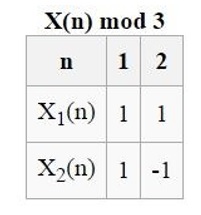
(though again this second calculation is superfluous since $\chi_2(1) = 1$ anyway). This completes the second character.

k = 5

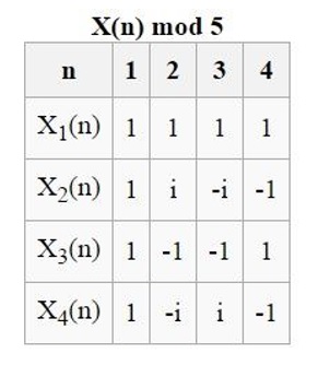
We have $\varphi(5) = 4$ so there are four Dirichlet characters in this case. We consider the four roots of unity

$\omega = e^{2 \pi i/4} = e^{\pi i/2} = i$

$\omega^2 = e^{4 \pi i/4} = e^{\pi i} = -1$

$\omega^3 = e^{6 \pi i/4} = e^{3 \pi i/2} = -i$

$\omega^4 = e^{8 \pi i/4} = e^{2 \pi i} = 1$

Note that the set of least positive residues mod $5$ is generated by $2$ :

$2 \equiv 2$ mod( $5$ )

$2^2 \equiv 4$ mod( $5$ )

$2^3 \equiv 3$ mod( $5$ )

$2^4 \equiv 1$ mod( $5$ )

Therefore the non-principal Dirichlet characters will be completely determined by the values of $\chi(2)$ . If we set

$\chi_2(2) = \omega = i$

then

$\chi_2(3) = \chi_2(2^3) = \chi_2^3(2) = -i$

$\chi_2(4) = \chi_2(2^2) = \chi_2^2(2) = -1$

(and we have $\chi_2(1) = 1$ ). This completes the second character.

To compute the third character we can set

$\chi_3(2) = \omega^2 = -1$

then

$\chi_3(3) = \chi_3(2^3) = \chi_3^3(2) = -1$

$\chi_3(4) = \chi_3(2^2) = \chi_3^2(2) = 1$

(and we have $\chi_3(1) = 1$ ). This completes the third character.

To compute the fourth character we set

$\chi_4(2) = \omega^3 = -i$

then

$\chi_4(3) = \chi_4(2^3) = \chi_4^3(2) = i$

$\chi_4(4) = \chi_4(2^2) = \chi_4^2(2) = -1$

(and we have $\chi_4(1) = 1$ ). This completes the fourth character.

k = 6

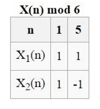
We have $\varphi(6) = 2$ so there are two Dirichlet characters in this case. We consider the two roots of unity

$\omega = e^{2 \pi i/2} = e^{\pi i} = -1$

and

$\omega^2 = 1$

Note that the set of least positive residues mod $6$ is generated by $5$ :

$5 \equiv 5$ mod( $6$ )

$5^2 \equiv 1$ mod( $6$ )

Therefore the non-principal Dirichlet character will be completely determined by the values of $\chi(5)$ . If we set

$\chi_2(5) = \omega = -1$

then

$\chi_2(1) = \chi_2(5^2) = \chi_2^2(5) = \omega^2 = 1$

(though again this second calculation is superfluous since $\chi_2(1) = 1$ anyway). This completes the second character.

k = 7

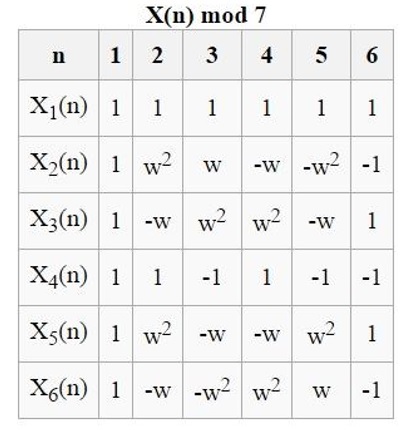
We have $\varphi(7) = 6$ so there are six Dirichlet characters in this case. We consider the six roots of unity

$\omega = e^{2 \pi i/6} = e^{\pi i/3}$

$\omega^2 = e^{2 \pi i/3}$

$\omega^3 = e^{3 \pi i/3} = e^{\pi i} = -1$

$\omega^4 = \omega \cdot \omega^3 = -\omega$

$\omega^5 = \omega \cdot \omega^4 = -\omega^2$

$\omega^6 = e^{6 \pi i/3} = e^{2\pi i} = 1$

Note that the set of least positive residues mod $7$ is generated by $3$ :

$3 \equiv 3$ mod( $7$ )

$3^2 \equiv 2$ mod( $7$ )

$3^3 \equiv 6$ mod( $7$ )

$3^4 \equiv 4$ mod( $7$ )

$3^5 \equiv 5$ mod( $7$ )

$3^6 \equiv 1$ mod( $7$ )

Therefore the non-principal Dirichlet characters will be completely determined by the values of $\chi(3)$ . If we set

$\chi_2(3) = \omega$

then

$\chi_2(2) = \chi_2(3^2) = \chi_2^2(3) = \omega^2$

$\chi_2(4) = \chi_2(3^4) = \chi_2^4(3) = \omega^4 = -\omega$

$\chi_2(5) = \chi_2(3^5) = \chi_2^5(3) = \omega^5 = -\omega^2$

$\chi_2(6) = \chi_2(3^3) = \chi_2^3(3) = \omega^3 = -1$

(and we have $\chi_2(1) = 1$ ). This completes the second character.

To compute the third character we can set

$\chi_3(3) = \omega^2$

then

$\chi_3(2) = \chi_3(3^2) = \chi_3^2(3) = \omega^4 = -\omega$

$\chi_3(4) = \chi_3(3^4) = \chi_3^4(3) = \omega^8 = \omega^2$

$\chi_3(5) = \chi_3(3^5) = \chi_3^5(3) = \omega^{10} = -\omega$

$\chi_3(6) = \chi_3(3^3) = \chi_3^3(3) = \omega^6 = 1$

(and we have $\chi_3(1) = 1$ ). This completes the third character.

To compute the fourth character we can set

$\chi_4(3) = \omega^3 = -1$

then

$\chi_4(2) = \chi_4(3^2) = \chi_4^2(3) = 1$

$\chi_4(4) = \chi_4(3^4) = \chi_4^4(3) = 1$

$\chi_4(5) = \chi_4(3^5) = \chi_4^5(3) = -1$

$\chi_4(6) = \chi_4(3^3) = \chi_4^3(3) = -1$

(and we have $\chi_4(1) = 1$ ). This completes the fourth character.

To compute the fifth character we can set

$\chi_5(3) = \omega^4 = -\omega$

then

$\chi_5(2) = \chi_5(3^2) = \chi_5^2(3) = \omega^2$

$\chi_5(4) = \chi_5(3^4) = \chi_5^4(3) = \omega^4 = -\omega$

$\chi_5(5) = \chi_5(3^5) = \chi_5^5(3) = \chi_5^4(3) \cdot \chi_5(3) = \omega^2$

$\chi_5(6) = \chi_5(3^3) = \chi_5^3(3) = -\omega^3 = 1$

(and we have $\chi_5(1) = 1$ ). This completes the fifth character.

Finally, to compute the sixth character we set

$\chi_6(3) = \omega^5 = -\omega^2$

then

$\chi_6(2) = \chi_6(3^2) = \chi_6^2(3) = \omega^4 = -\omega$

$\chi_6(4) = \chi_6(3^4) = \chi_6^4(3) = \omega^8 = \omega^2$

$\chi_6(5) = \chi_6(3^5) = \chi_6^5(3) = -\omega^{10} = \omega$

$\chi_6(6) = \chi_6(3^3) = \chi_6^3(3) = -\omega^6 = -1$

(and we have $\chi_6(1) = 1$ ). This completes the sixth character.

k = 8

We have $\varphi(8) = 4$ so there are four Dirichlet characters in this case. We consider the four roots of unity

$\omega = e^{2 \pi i/4} = e^{\pi i/2} = i$

$\omega^2 = e^{4 \pi i/4} = e^{\pi i} = -1$

$\omega^3 = e^{6 \pi i/4} = e^{3 \pi i/2} = -i$

$\omega^4 = e^{8 \pi i/4} = e^{2 \pi i} = 1$

In this case, none of the four elements of the set of least positive residues mod $8$ generates the entire set. However, the characters must satisfy the following relations, which restrict the choices:

$\chi(3) \cdot \chi(5) = \chi(15) = \chi(7)$

$\chi(3) \cdot \chi(7) = \chi(21) = \chi(5)$

$\chi(5) \cdot \chi(7) = \chi(35) = \chi(3)$

Each character’s values must be chosen in such a way that these three relations hold.

To compute the second character, suppose we begin by trying to set

$\chi_2(3) = \omega = i$

and

$\chi_2(5) = \omega^2 = -1$

Then we must have

$\chi_2(7) = \chi_2(3) \cdot \chi_2(5) = -i$

but then

$\chi_2(3) \cdot \chi_2(7) = 1 \neq \chi_2(5)$

so this does not work. If instead we try to set

$\chi_2(5) = -i$

then we must have

$\chi_2(7) = \chi_2(3) \cdot \chi_2(5) = 1$

but then

$\chi_2(3) \cdot \chi_2(7) = i \neq \chi_2(5)$

so this does not work either. Computations like these show that $\pm i$ cannot appear in any of the characters mod $8$ . All the characters must be formed from $\pm 1$ . (Fundamentally, this is due to the fact that the group of least positive residues mod $8$ can be subdivided into four cyclic subgroups of order 2, each of which has characters whose values are the two roots of unity, $1$ and $-1$ ).

To compute the second character we can set

$\chi_2(3) = 1$

and

$\chi_2(5) = -1$

then we must have

$\chi_2(7) = -1$

and this works.

To compute the third character we can set

$\chi_3(3) = -1$

and

$\chi_3(5) = -1$

then we must have

$\chi_3(7) = 1$

and this works too.

Finally, to compute the fourth character we can set

$\chi_4(3) = -1$

and

$\chi_4(5) = 1$

then we must have

$\chi_4(7) = -1$

and this works too.

k = 9

We have $\varphi(9) = 6$ so there are six Dirichlet characters in this case. We consider the six roots of unity

$\omega = e^{2 \pi i/6} = e^{\pi i/3}$

$\omega^2 = e^{2 \pi i/3}$

$\omega^3 = e^{3 \pi i/3} = e^{\pi i} = -1$

$\omega^4 = \omega \cdot \omega^3 = -\omega$

$\omega^5 = \omega \cdot \omega^4 = -\omega^2$

$\omega^6 = e^{6 \pi i/3} = e^{2\pi i} = 1$

Note that the set of least positive residues mod $9$ is generated by $2$ :

$2 \equiv 2$ mod( $9$ )

$2^2 \equiv 4$ mod( $9$ )

$2^3 \equiv 8$ mod( $9$ )

$2^4 \equiv 7$ mod( $9$ )

$2^5 \equiv 5$ mod( $9$ )

$2^6 \equiv 1$ mod( $9$ )

Therefore the non-principal Dirichlet characters will be completely determined by the values of $\chi(2)$ . If we set

$\chi_2(2) = \omega$

then

$\chi_2(4) = \chi_2(2^2) = \chi_2^2(2) = \omega^2$

$\chi_2(5) = \chi_2(2^5) = \chi_2^5(2) = \omega^5 = -\omega^2$

$\chi_2(7) = \chi_2(2^4) = \chi_2^4(2) = \omega^4 = -\omega$

$\chi_2(8) = \chi_2(2^3) = \chi_2^3(2) = \omega^3 = -1$

(and we have $\chi_2(1) = 1$ ). This completes the second character.

To compute the third character we can set

$\chi_3(2) = \omega^2$

then

$\chi_3(4) = \chi_3(2^2) = \chi_3^2(2) = \omega^4 = -\omega$

$\chi_3(5) = \chi_3(2^5) = \chi_3^5(2) = \omega^{10} = \omega^6 \cdot \omega^4 = -\omega$

$\chi_3(7) = \chi_3(2^4) = \chi_3^4(2) = \omega^8 = \omega^6 \cdot \omega^2 = \omega^2$

$\chi_3(8) = \chi_3(2^3) = \chi_3^3(2) = \omega^6 = 1$

(and we have $\chi_3(1) = 1$ ). This completes the third character.

To compute the fourth character we can set

$\chi_4(2) = \omega^3 = -1$

then

$\chi_4(4) = \chi_4(2^2) = \chi_4^2(2) = 1$

$\chi_4(5) = \chi_4(2^5) = \chi_4^5(2) = -1$

$\chi_4(7) = \chi_4(2^4) = \chi_4^4(2) = 1$

$\chi_4(8) = \chi_4(2^3) = \chi_4^3(2) = -1$

(and we have $\chi_4(1) = 1$ ). This completes the fourth character.

To compute the fifth character we can set

$\chi_5(2) = \omega^4 = -\omega$

then

$\chi_5(4) = \chi_5(2^2) = \chi_5^2(2) = \omega^2$

$\chi_5(5) = \chi_5(2^5) = \chi_5^5(2) = -\omega^5 = -\omega^3 \cdot \omega^2 = \omega^2$

$\chi_5(7) = \chi_5(2^4) = \chi_5^4(2) = \omega^4 = \omega^3 \cdot \omega = -\omega$

$\chi_5(8) = \chi_5(2^3) = \chi_5^3(2) = -\omega^3 = 1$

(and we have $\chi_5(1) = 1$ ). This completes the fifth character.

Finally, to compute the sixth character we can set

$\chi_6(2) = \omega^5 = -\omega^2$

then

$\chi_6(4) = \chi_6(2^2) = \chi_6^2(2) = \omega^4 = -\omega$

$\chi_6(5) = \chi_6(2^5) = \chi_6^5(2) = -\omega^{10} = -\omega^6 \cdot \omega^4 = \omega$

$\chi_6(7) = \chi_6(2^4) = \chi_6^4(2) = \omega^8 = \omega^6 \cdot \omega^2 = \omega^2$

$\chi_6(8) = \chi_6(2^3) = \chi_6^3(2) = -\omega^6 = -1$

(and we have $\chi_6(1) = 1$ ). This completes the sixth character.

k = 10

We have $\varphi(10) = 4$ so there are four Dirichlet characters in this case. We consider the four roots of unity

$\omega = e^{2 \pi i/4} = e^{\pi i/2} = i$

$\omega^2 = e^{4 \pi i/4} = e^{\pi i} = -1$

$\omega^3 = e^{6 \pi i/4} = e^{3 \pi i/2} = -i$

$\omega^4 = e^{8 \pi i/4} = e^{2 \pi i} = 1$

Note that the set of least positive residues mod $10$ is generated by $3$ :

$3 \equiv 3$ mod( $10$ )

$3^2 \equiv 9$ mod( $10$ )

$3^3 \equiv 7$ mod( $10$ )

$3^4 \equiv 1$ mod( $10$ )

Therefore the non-principal Dirichlet characters will be completely determined by the values of $\chi(3)$ . If we set

$\chi_2(3) = \omega = i$

then

$\chi_2(7) = \chi_2(3^3) = \chi_2^3(3) = -i$

$\chi_2(9) = \chi_2(3^2) = \chi_2^2(3) = -1$

(and we have $\chi_2(1) = 1$ ). This completes the second character.

To compute the third character we can set

$\chi_3(3) = \omega^2 = -1$

then

$\chi_3(7) = \chi_3(3^3) = \chi_3^3(3) = -1$

$\chi_3(9) = \chi_3(3^2) = \chi_3^2(3) = 1$

(and we have $\chi_3(1) = 1$ ). This completes the third character.

Finally, to compute the fourth character we set

$\chi_4(3) = \omega^3 = -i$

then

$\chi_4(7) = \chi_4(3^3) = \chi_4^3(3) = i$

$\chi_4(9) = \chi_4(3^2) = \chi_4^2(3) = -1$

(and we have $\chi_4(1) = 1$ ). This completes the fourth character.

k = 11

We have $\varphi(11) = 10$ so there are ten Dirichlet characters in this case. We consider the ten roots of unity

$\omega = e^{2 \pi i/10} = e^{\pi i/5}$

$\omega^2 = e^{2 \pi i/5}$

$\omega^3 = e^{3 \pi i/5}$

$\omega^4 = e^{4 \pi i/5}$

$\omega^5 = e^{5 \pi i/5} = e^{\pi i} = -1$

$\omega^6 = -\omega$

$\omega^7 = -\omega^2$

$\omega^8 = -\omega^3$

$\omega^9 = -\omega^4$

$\omega^{10} = -\omega^5 = 1$

Note that the set of least positive residues mod $11$ is generated by $2$ :

$2 \equiv 2$ mod( $11$ )

$2^2 \equiv 4$ mod( $11$ )

$2^3 \equiv 8$ mod( $11$ )

$2^4 \equiv 5$ mod( $11$ )

$2^5 \equiv 10$ mod( $11$ )

$2^6 \equiv 9$ mod( $11$ )

$2^7 \equiv 7$ mod( $11$ )

$2^8 \equiv 3$ mod( $11$ )

$2^9 \equiv 6$ mod( $11$ )

$2^{10} \equiv 1$ mod( $11$ )

Therefore the non-principal Dirichlet characters will be completely determined by the values of $\chi(2)$ . If we set

$\chi_2(2) = \omega$

then

$\chi_2(3) = \chi_2(2^8) = \chi_2^8(2) = \omega^8 = -\omega^3$

$\chi_2(4) = \chi_2(2^2) = \chi_2^2(2) = \omega^2$

$\chi_2(5) = \chi_2(2^4) = \chi_2^4(2) = \omega^4$

$\chi_2(6) = \chi_2(2^9) = \chi_2^9(2) = \omega^9 = -\omega^4$

$\chi_2(7) = \chi_2(2^7) = \chi_2^7(2) = \omega^7 = -\omega^2$

$\chi_2(8) = \chi_2(2^3) = \chi_2^3(2) = \omega^3$

$\chi_2(9) = \chi_2(2^6) = \chi_2^6(2) = \omega^6 = -\omega$

$\chi_2(10) = \chi_2(2^5) = \chi_2^5(2) = \omega^5 = -1$

(and we have $\chi_2(1) = 1$ ). This completes the second character.

To compute the third character we can set

$\chi_3(2) = \omega^2$

then

$\chi_3(3) = \chi_3(2^8) = \chi_3^8(2) = \omega^{16} = -\omega$

$\chi_3(4) = \chi_3(2^2) = \chi_3^2(2) = \omega^4$

$\chi_3(5) = \chi_3(2^4) = \chi_3^4(2) = \omega^8 = -\omega^3$

$\chi_3(6) = \chi_3(2^9) = \chi_3^9(2) = \omega^{18} = -\omega^3$

$\chi_3(7) = \chi_3(2^7) = \chi_3^7(2) = \omega^{14} = \omega^4$

$\chi_3(8) = \chi_3(2^3) = \chi_3^3(2) = \omega^6 = -\omega$

$\chi_3(9) = \chi_3(2^6) = \chi_3^6(2) = \omega^{12} = \omega^2$

$\chi_3(10) = \chi_3(2^5) = \chi_3^5(2) = \omega^{10} = 1$

(and we have $\chi_3(1) = 1$ ). This completes the third character.

To compute the fourth character we can set

$\chi_4(2) = \omega^3$

then

$\chi_4(3) = \chi_4(2^8) = \chi_4^8(2) = \omega^{24} = \omega^4$

$\chi_4(4) = \chi_4(2^2) = \chi_4^2(2) = \omega^6 = -\omega$

$\chi_4(5) = \chi_4(2^4) = \chi_4^4(2) = \omega^{12} = \omega^2$

$\chi_4(6) = \chi_4(2^9) = \chi_4^9(2) = \omega^{27} = -\omega^2$

$\chi_4(7) = \chi_4(2^7) = \chi_4^7(2) = \omega^{21} = \omega$

$\chi_4(8) = \chi_4(2^3) = \chi_4^3(2) = \omega^9 = -\omega^4$

$\chi_4(9) = \chi_4(2^6) = \chi_4^6(2) = \omega^{18} = -\omega^3$

$\chi_4(10) = \chi_4(2^5) = \chi_4^5(2) = \omega^{15} = -1$

(and we have $\chi_4(1) = 1$ ). This completes the fourth character.

To compute the fifth character we can set

$\chi_5(2) = \omega^4$

then

$\chi_5(3) = \chi_5(2^8) = \chi_5^8(2) = \omega^{32} = \omega^2$

$\chi_5(4) = \chi_5(2^2) = \chi_5^2(2) = \omega^8 = -\omega^3$

$\chi_5(5) = \chi_5(2^4) = \chi_5^4(2) = \omega^{16} = -\omega$

$\chi_5(6) = \chi_5(2^9) = \chi_5^9(2) = \omega^{36} = -\omega$

$\chi_5(7) = \chi_5(2^7) = \chi_5^7(2) = \omega^{28} = -\omega^3$

$\chi_5(8) = \chi_5(2^3) = \chi_5^3(2) = \omega^{12} = \omega^2$

$\chi_5(9) = \chi_5(2^6) = \chi_5^6(2) = \omega^{24} = \omega^4$

$\chi_5(10) = \chi_5(2^5) = \chi_5^5(2) = \omega^{20} = 1$

(and we have $\chi_5(1) = 1$ ). This completes the fifth character.

To compute the sixth character we can set

$\chi_6(2) = \omega^5 = -1$

then

$\chi_6(3) = \chi_6(2^8) = \chi_6^8(2) = 1$

$\chi_6(4) = \chi_6(2^2) = \chi_6^2(2) = 1$

$\chi_6(5) = \chi_6(2^4) = \chi_6^4(2) = 1$

$\chi_6(6) = \chi_6(2^9) = \chi_6^9(2) = -1$

$\chi_6(7) = \chi_6(2^7) = \chi_6^7(2) = -1$

$\chi_6(8) = \chi_6(2^3) = \chi_6^3(2) = -1$

$\chi_6(9) = \chi_6(2^6) = \chi_6^6(2) = 1$

$\chi_6(10) = \chi_6(2^5) = \chi_6^5(2) = -1$

(and we have $\chi_6(1) = 1$ ). This completes the sixth character.

To compute the seventh character we can set

$\chi_7(2) = \omega^6 = -\omega$

then

$\chi_7(3) = \chi_7(2^8) = \chi_7^8(2) = \omega^8 = -\omega^3$

$\chi_7(4) = \chi_7(2^2) = \chi_7^2(2) = \omega^2$

$\chi_7(5) = \chi_7(2^4) = \chi_7^4(2) = \omega^4$

$\chi_7(6) = \chi_7(2^9) = \chi_7^9(2) = -\omega^9 = \omega^4$

$\chi_7(7) = \chi_7(2^7) = \chi_7^7(2) = -\omega^7 = \omega^2$

$\chi_7(8) = \chi_7(2^3) = \chi_7^3(2) = -\omega^3$

$\chi_7(9) = \chi_7(2^6) = \chi_7^6(2) = \omega^6 = -\omega$

$\chi_7(10) = \chi_7(2^5) = \chi_7^5(2) = -\omega^5 = 1$

(and we have $\chi_7(1) = 1$ ). This completes the seventh character.

To compute the eighth character we can set

$\chi_8(2) = \omega^7 = -\omega^2$

then

$\chi_8(3) = \chi_8(2^8) = \chi_8^8(2) = \omega^{16} = -\omega$

$\chi_8(4) = \chi_8(2^2) = \chi_8^2(2) = \omega^4$

$\chi_8(5) = \chi_8(2^4) = \chi_8^4(2) = \omega^8 = -\omega^3$

$\chi_8(6) = \chi_8(2^9) = \chi_8^9(2) = -\omega^{18} = \omega^3$

$\chi_8(7) = \chi_8(2^7) = \chi_8^7(2) = -\omega^{14} = -\omega^4$

$\chi_8(8) = \chi_8(2^3) = \chi_8^3(2) = -\omega^6 = \omega$

$\chi_8(9) = \chi_8(2^6) = \chi_8^6(2) = \omega^{12} = \omega^2$

$\chi_8(10) = \chi_8(2^5) = \chi_8^5(2) = -\omega^{10} = -1$

(and we have $\chi_8(1) = 1$ ). This completes the eighth character.

To compute the ninth character we can set

$\chi_9(2) = \omega^8 = -\omega^3$

then

$\chi_9(3) = \chi_9(2^8) = \chi_9^8(2) = \omega^{24} = \omega^4$

$\chi_9(4) = \chi_9(2^2) = \chi_9^2(2) = \omega^6 = -\omega$

$\chi_9(5) = \chi_9(2^4) = \chi_9^4(2) = \omega^{12} = \omega^2$

$\chi_9(6) = \chi_9(2^9) = \chi_9^9(2) = -\omega^{27} = \omega^2$

$\chi_9(7) = \chi_9(2^7) = \chi_9^7(2) = -\omega^{21} = -\omega$

$\chi_9(8) = \chi_9(2^3) = \chi_9^3(2) = -\omega^9 = \omega^4$

$\chi_9(9) = \chi_9(2^6) = \chi_9^6(2) = \omega^{18} = -\omega^3$

$\chi_9(10) = \chi_9(2^5) = \chi_9^5(2) = -\omega^{15} = 1$

(and we have $\chi_9(1) = 1$ ). This completes the ninth character.

Finally, to compute the tenth character we set

$\chi_{10}(2) = \omega^9 = -\omega^4$

then

$\chi_{10}(3) = \chi_{10}(2^8) = \chi_{10}^8(2) = \omega^{32} = \omega^2$

$\chi_{10}(4) = \chi_{10}(2^2) = \chi_{10}^2(2) = \omega^8 = -\omega^3$

$\chi_{10}(5) = \chi_{10}(2^4) = \chi_{10}^4(2) = \omega^{16} = -\omega$

$\chi_{10}(6) = \chi_{10}(2^9) = \chi_{10}^9(2) = -\omega^{36} = \omega$

$\chi_{10}(7) = \chi_{10}(2^7) = \chi_{10}^7(2) = -\omega^{28} = \omega^3$

$\chi_{10}(8) = \chi_{10}(2^3) = \chi_{10}^3(2) = -\omega^{12} = -\omega^2$

$\chi_{10}(9) = \chi_{10}(2^6) = \chi_{10}^6(2) = \omega^{24} = \omega^4$

$\chi_{10}(10) = \chi_{10}(2^5) = \chi_{10}^5(2) = -\omega^{20} = -1$

(and we have $\chi_{10}(1) = 1$ ). This completes the tenth character.

Invariance under rotations in space and conservation of angular momentum

In a previous note I studied the mathematical setup of Noether’s Theorem and its proof. I briefly illustrated the mathematical machinery by considering invariance under translations in time, giving the law of conservation of energy, and invariance under translations in space, giving the law of conservation of linear momentum. I briefly mentioned that invariance under rotations in space would also yield the law of conservation of angular momentum but I did not work this out explicitly. I want to quickly do this in the present note.

We imagine a particle of unit mass moving freely in the absence of any potential field, and tracing out a path $\gamma(t)$ in the $(x, y)$ -plane of a three-dimensional Euclidean coordinate system between times $t_1$ and $t_2$ , with the $z$ -coordinate everywhere zero along this path. The angular momentum of the particle at time $t$ with respect to the origin of the coordinate system is given by

$\mathbf{L} = \mathbf{r} \times \mathbf{v}$

$= (\mathbf{i} x + \mathbf{j} y) \times (\mathbf{i} \dot{x} + \mathbf{j} \dot{y})$

$= \mathbf{k} x \dot{y} - \mathbf{k} y \dot{x}$

$= \mathbf{k} (x \dot{y} - y \dot{x})$

where $\times$ is the vector product operation. Alternatively, we could have obtained this as

$\mathbf{L} = \mathbf{r} \times \mathbf{v} = \begin{vmatrix} \mathbf{i} & \mathbf{j} & \mathbf{k} \\ \ \\x & y & 0 \\ \ \\ \dot{x} & \dot{y} & 0 \end{vmatrix}$

$= \mathbf{k} (x \dot{y} - y \dot{x})$

In terms of Lagrangian mechanics, the path $\gamma(t)$ followed by the particle will be a stationary path of the action functional

$S[\gamma(t)] = \int_{t_1}^{t_2} dt \frac{1}{2}(\dot{x}^2 + \dot{y}^2)$

(in the absence of a potential field the total energy consists only of kinetic energy).

Now imagine that the entire path $\gamma(t)$ is rotated bodily anticlockwise in the $(x, y)$ -plane through an angle $\theta$ . This corresponds to a one-parameter transformation

$\overline{t} \equiv \Phi(t, x, y, \dot{x}, \dot{y}; \theta) = t$

$\overline{x} \equiv \Psi_1(t, x, y, \dot{x}, \dot{y}; \theta) = x \cos \theta - y \sin \theta$

$\overline{y} \equiv \Psi_2(t, x, y, \dot{x}, \dot{y}; \theta) = x \sin \theta + y \cos \theta$

which reduces to the identity when $\theta = 0$ . We have

$d\overline{t} = dt$

$\dot{\overline{x}}^2 = \dot{x}^2 \cos^2 \theta + \dot{y}^2 \sin^2 \theta - 2 \dot{x} \dot{y} \sin \theta \cos \theta$

$\dot{\overline{y}}^2 = \dot{x}^2 \sin^2 \theta + \dot{y}^2 \cos^2 \theta + 2 \dot{x} \dot{y} \sin \theta \cos \theta$

and therefore

$\dot{x}^2 + \dot{y}^2 = \dot{\overline{x}}^2 + \dot{\overline{y}}^2$

so the action functional is invariant under this rotation since

$S[\overline{\gamma}(t)] = \int_{t_1}^{t_2} d\overline{t} \frac{1}{2}(d\dot{\overline{x}}^2 + d\dot{\overline{y}}^2) = \int_{t_1}^{t_2} dt \frac{1}{2}(\dot{x}^2 + \dot{y}^2) = S[\gamma(t)]$

Therefore Noether’s theorem applies. Let

$F(t, x, y, \dot{x}, \dot{y}) = \frac{1}{2}(\dot{x}^2 + \dot{y}^2)$

Then Noether’s theorem in this case says

$\frac{\partial F}{\partial \dot{x}} \psi_1 + \frac{\partial F}{\partial \dot{y}} \psi_2 + \big(F - \frac{\partial F}{\partial \dot{x}} \dot{x} - \frac{\partial F}{\partial \dot{y}} \dot{y}\big) \phi = const.$

where

$\phi \equiv \frac{\partial \Phi}{\partial \theta} \big|_{\theta = 0} = 0$

$\psi_1 \equiv \frac{\partial \Psi_1}{\partial \theta} \big|_{\theta = 0} = -y$

$\psi_2 \equiv \frac{\partial \Psi_2}{\partial \theta} \big|_{\theta = 0} = x$

We have

$\frac{\partial F}{\partial \dot{x}} = \dot{x}$

$\frac{\partial F}{\partial \dot{y}} = \dot{y}$

Therefore Noether’s theorem gives us (remembering $\phi = 0$ )

$-\dot{x} y + \dot{y} x = const.$

The expression on the left-hand side of this equation is the angular momentum of the particle (cf. the brief discussion of angular momentum at the start of this note), so this result is precisely the statement that the angular momentum is conserved. Noether’s theorem shows us that this is a direct consequence of the invariance of the action functional of the particle under rotations in space.