Dr Christian P. H. Salas

In the present post I want to record some notes I made on the mathematical nuances involved in a proof of Noether’s theorem and the mathematical relevance of the theorem to some simple conservation laws in classical physics, namely, the conservation of energy and the conservation of linear momentum. Noether’s Theorem has important applications in a wide range of classical mechanics problems as well as in quantum mechanics and Einstein’s relativity theory. It is also used in the study of certain classes of partial differential equations that can be derived from variational principles.

The theorem was first published by Emmy Noether in 1918. An interesting book by Yvette Kosmann-Schwarzbach presents an English translation of Noether’s 1918 paper and discusses in detail the history of the theorem’s development and its impact on theoretical physics in the 20th Century. (Kosmann-Schwarzbach, Y, 2011, The Noether Theorems: Invariance and Conservation Laws in the Twentieth Century. Translated by Bertram Schwarzbach. Springer). At the time of writing, the book is freely downloadable online.

Mathematical setup of Noether’s theorem

The case I explore in detail here is that of a variational calculus functional of the form

where is a single independent variable and is a vector of dependent variables. The functional has stationary paths defined by the usual Euler-Lagrange equations of variational calculus. Noether’s theorem concerns how the value of this functional is affected by families of continuous transformations of the dependent and independent variables (e.g., translations, rotations) that are defined in terms of one or more real parameters. The case I explore in detail here involves transformations defined in terms of only a single parameter, call it . The transformations can be represented in general terms as

for . The functions and are assumed to have continuous first derivatives with respect to all the variables, including the parameter . Furthermore, the transformations must reduce to identities when , i.e.,

for . As concrete examples, translations and rotations are continuous differentiable transformations that can be defined in terms of a single parameter and that reduce to identities when the parameter takes the value zero.

Noether’s theorem is assumed to apply to infinitesimally small changes in the dependent and independent variables, so we can assume and then use perturbation theory to prove the theorem. Treating and as functions of and Taylor-expanding them about we get

where

and

where

for .

Noether’s theorem then says that whenever the functional is invariant under the above family of transformations, i.e., whenever

for all and such that , where and , then for each stationary path of the following equation holds:

As illustrated below, this remarkable equation encodes a number of conservation laws in physics, including conservation of energy, linear and angular momentum given that the relevant equations of motion are invariant under translations in time and space, and under rotations in space respectively. Thus, Noether’s theorem is often expressed as a statement along the lines that whenever a system has a continuous symmetry there must be corresponding quantities whose values are conserved.

Application of the theorem to familiar conservation laws in classical physics

It is, of course, not necessary to use the full machinery of Noether’s theorem for simple examples of conservation laws in classical physics. The theorem is most useful in unfamiliar situations in which it can reveal conserved quantities which were not previously known. However, going through the motions in simple cases clarifies how the mathematical machinery works in more sophisticated and less familiar situations.

To obtain the law of the conservation of energy in the simplest possible scenario, consider a particle of mass moving along a straight line in a time-invariant potential field with position at time given by the function . The Lagrangian formulation of mechanics then says that the path followed by the particle will be a stationary path of the action functional

The Euler-Lagrange equation for this functional would give Newton’s second law as the equation governing the particle’s motion. With regard to demonstrating energy conservation, we notice that the Lagrangian, which is more generally of the form when there is a time-varying potential, here takes the simpler form because there is no explicit dependence on time. Therefore we might expect the functional to be invariant under translations in time, and thus Noether’s theorem to hold. We will verify this. In the context of the mathematical setup of Noether’s theorem above, we can write the relevant transformations as

and

From the first equation we see that in the case of a simple translation in time by an amount , and from the second equation we see that , which simply reflects the fact that we are only translating in the time direction. The invariance of the functional under these transformations can easily be demonstrated by writing

where the limits in the second integral follow from the change of the time variable from to . Thus, Noether’s theorem holds and with  and  the fundamental equation in the theorem reduces to

Evaluating the terms on the left-hand side we get

which is of course the statement of the conservation of energy.

To obtain the law of conservation of linear momentum in the simplest possible scenario, assume now that the above particle is moving freely in the absence of any potential field, so and the only energy involved is kinetic energy. The path followed by the particle will now be a stationary path of the action functional

The Euler-Lagrange equation for this functional would give Newton’s first law as the equation governing the particle’s motion (constant velocity in the absence of any forces). To get the law of conservation of linear momentum we will consider a translation in space rather than time, and check that the action functional is invariant under such translations. In the context of the mathematical setup of Noether’s theorem above, we can write the relevant transformations as

and

From the first equation we see that reflecting the fact that we are only translating in the space direction, and from the second equation we see that in the case of a simple translation in space by an amout . The invariance of the functional under these transformations can easily be demonstrated by noting that , so we can write

since the limits of integration are not affected by the translation in space. Thus, Noether’s theorem holds and with  and  the fundamental equation in the theorem reduces to

This is, of course, the statement of the conservation of linear momentum.

Proof of Noether’s theorem

To prove Noether’s theorem we will begin with the transformed functional

We will substitute into this the linearised forms of the transformations, namely

and

for , and then expand to first order in . Note that the integration limits are, to first order in ,

and

Using the linearised forms of the transformations and writing we get

Inverting the second equation we get

Using this in the first equation we find, to first order in ,

Making the necessary substitutions we can then write the transformed functional as

Treating as a function of and expanding about to first order we get

Then using the expression for  above, the transformed functional becomes

Ignoring the second order term in we can thus write

Since the functional is invariant, however, this implies

We now manipulate this equation by integrating the terms involving  and by parts. We get

and

Substituting these into the equation gives

We can manipulate this equation further by expanding the integrand in the second term on the left-hand side. We get

Thus, the equation becomes

We can now see at a glance that the second and third terms on the left-hand side must vanish because of the Euler-Lagrange expressions appearing in the brackets (which are identically zero on stationary paths). Thus we arrive at the equation

which proves that the formula inside the square brackets is constant as per Noether’s theorem.

A geodesic can be defined as an extremal path between two points on a manifold in the sense that it minimises or maximises some criterion of interest (e.g., minimises distance travelled, maximises proper time, etc). Such a path will satisfy some geodesic equations equivalent to the Euler-Lagrange equations of the calculus of variations. A geodesic can also be defined in a conceptually different way as the straightest possible path between two points on a manifold. In this case the path will satisfy geodesic equations derived by requiring parallel transport of a tangent vector along the path. Although these are conceptually different ways of defining geodesics, they are mathematically equivalent. In the present note I want to explore the derivation of geodesic equations in these two different ways and prove their mathematical equivalence.

Now, in the calculus of variations we typically define a system’s action to be the time-integral of a Lagrangian :

where says that the Lagrangian is a function of position coordinates and velocities (and ranges over however many coordinates there are). We find the trajectory that yields a desired extremal value of the action as the one that satisfies the Euler-Lagrange equations

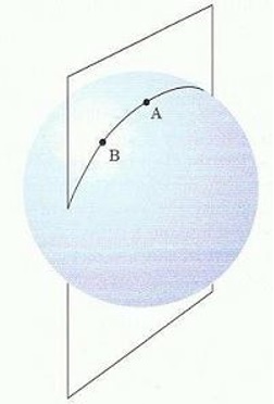
Let us now suppose that we are facing an exactly analogous situation in which there are two points on the manifold, and , and we are considering possible paths between them to try to find the extremal one. We can describe any path between and by specifying the coordinates of the points along it as functions of a parameter that goes from a value of at to a value of at , i.e., by specifying the functions . Noting that the line element can be written as

we can write the length of a particular path as

Note that the metric is a function of the coordinates of points along the path, which in turn are functions of the parameter , i.e., . This situation is exactly analogous to the usual calculus of variations scenario because, writing , we see that we have a Lagrangian function

and we hope to find the path that makes the integral of the Lagrangian extreme. This will be the path that satisfies the Euler-Lagrange equations

This corresponds to separate differential equations in an -dimensional manifold, one equation for each value of the index .

We can manipulate the Euler-Lagrange equations to get geodesic equations which are easier to use in particular contexts. First, note that

because, for example, . Also note that the metric is treated as a constant as it depends on not on . Doing the sums over the Kronecker deltas we get

But notice that since

we have

so

and we can write

Next, we have

Putting these results into the Euler-Lagrange equations we get

Finally, multiplying through by we get

where I have also renamed in the first term to make it clearer that the Einstein summations in the first and second terms are independent. This is the first version of the geodesic equations, derived by requiring that the path between the points and should be extremal in the sense of satisfying the Euler-Lagrange equations of the calculus of variations.

We will now derive a second version of the geodesic equations by requiring the geodesic to be a path that is locally straight. In differential geometry a path is defined as straight if it parallel transports its own tangent vector, i.e., if the tangent vector does not change as we move an infinitesimal step along the path. If we take an arbitrary point on the path to be and we take to be an infinitesimal displacement along the path, then a tangent vector to the path is

and we want

Multiplying through by this gives

But

Putting this into the equation gives

To enable us to factor out the basis vector we can rename the indices in the second term as and to get

This is the second version of the geodesic equations, derived by assuming that the path between the two points on the manifold is locally straight.

We now have two seemingly different versions of the geodesic equations, namely

and

We will next show that they are in fact mathematically equivalent. Starting from the first version, we can expand out the brackets to get

Now we rename the indices as follows: in the first term; in the second term; and in the third term; and , , in the fourth term. We get

We can write this as

Finally, multiplying through by and using the facts that

and

we get

which is the second version of the geodesic equation. Thus, the two versions are equivalent as claimed.

It is a delightful fact that one can get both the fundamental equation of classical mechanics (Newton’s Second Law) and the fundamental equation of quantum mechanics (Schrödinger’s equation) by solving very simple variational problems based on the familiar conservation of mechanical energy equation

In the present note I want to briefly set out the relevant calculations in a unified way emphasising the common underlying structure provided by the conservation of mechanical energy and the Calculus of Variations. The kinetic energy will be taken to be

where is the particle’s velocity, is its momentum, and is its mass. The potential energy will be regarded as some function of only.

To obtain Newton’s Second Law we find the stationary path followed by the particle with respect to the functional

The function is usually termed the Lagrangian in classical mechanics. The functional is usually called the action. The Euler-Lagrange equation for this Calculus of Variations problem is

and this is Newton’s Second Law in disguise! We have

and

so substituting these into the Euler-Lagrange equation we get Newton’s Second Law, .

To obtain Schrödinger’s equation we introduce a function

where is again the momentum of the particle and is the reduced Planck’s constant from quantum mechanics. (Note that has units of so we need to remove these by dividing by which has the same units, as the function in quantum mechanics is dimensionless). We then have

and differentiating both sides gives

so

Therefore we can write the kinetic energy as

and putting this into the conservation of mechanical energy equation gives

We now find the stationary path followed by the particle with respect to the functional

The Euler-Lagrange equation for this Calculus of Variations problem is

and this is Schrödinger’s equation in disguise! We have

and

so substituting these into the Euler-Lagrange equation we get

and this is the (time-independent) Schrödinger equation for a particle of mass with fixed total energy in a potential on the line .

A particle of mass with position vector and velocity (with respect to some specified origin) has a linear momentum vector and angular momentum vector

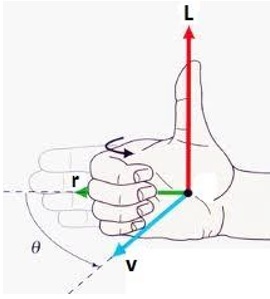
where is the vector product operation. The magnitude of the angular momentum vector is where is the angle between and . The direction of is given by the right-hand rule when the vectors and are placed with their tails at the same point: one curls the fingers of the right hand in the direction of rotation of into and the thumb then points in the direction of .

One can find the components of in the , and directions in Cartesian coordinates using

Therefore the components of in Cartesian coordinates are

In classical mechanics the angular momentum magnitude can take a continuum of values but in quantum mechanics only certain discrete values for are permissible. Furthermore, the linear momentum vector appearing in must obey Heisenberg’s uncertainty principle in each direction, i.e.,

in the -direction and similarly for the and directions. These features of quantized variables like and make it necessary to do calculations with them in quantum mechanics using their operator representations. (For example, on the quantum scale one cannot calculate the expectation of momentum in the direction using an integral involving momentum as a function of because no such function can exist: Heisenberg’s uncertainty principle prevents accurate knowledge of momentum when the value of is known exactly. One must therefore use the operator representation of momentum rather than momentum as some function of in order to calculate the expectation). It is a basic postulate of quantum mechanics that every observable quantity characterising a physical system can be represented by a quantum mechanical operator obtained by expressing the quantity in terms of and and then replacing the vector by where

and its components , and by

Taking this on board we can then write and , and in quantum mechanical operator form in Cartesian coordinates as

In order to perform some calculations involving Schrödinger’s equation I needed to employ the square of the quantum mechanical angular momentum operator , but in spherical polar coordinates rather than Cartesian coordinates, where

I used the matrix calculus approach in my previous note to achieve the necessary change of variables in . In the present note I want to record the details of this calculation as I have never seen this approach used elsewhere. (This change of variables can also be done using a scale factor method based on vector calculus which I will not go into here).

As in my previous note we begin the matrix calculus approach with the standard conversion equations for spherical polar coordinates:

Differentiating with respect to the vector we get

We can then use the matrix version of the chain rule to write

We can solve this system by inverting the coefficient matrix to get

Using the equations in this system together with the standard conversion equations we then have

and

Subtracting the second expression from the first and ignoring the in the numerators of the partial derivatives we can then write the angular momentum operator in the direction in terms of spherical polar coordinates as

Similarly we have

and

Therefore

Finally, we have

and

Therefore

Having obtained the components of in spherical polar coordinates we can now finally calculate the operator representation of as

In three-dimensional rectangular coordinates, the partial differential equation known as Laplace’s equation takes the form

This equation is applicable to a wide range of problems in physics but it is often necessary to make a change of variables from rectangular to spherical polar coordinates in order to better match the spherical symmetry of particular contexts. One can work out this change of variables using a scale factor method based on the formula for the Laplacian of a function in general orthogonal curvilinear coordinates:

This formula is derived using basic results from vector calculus and allows Laplace’s equation to be easily expressed in any orthogonal coordinate system once the form of the Euclidean metric is known in that coordinate system. (Orthogonal coordinate systems are those for which the coordinate basis vectors are always orthogonal at each point). The Euclidean metric in general orthogonal coordinates , , will take the form

The coefficients , and are the scale factors appearing in the Laplacian formula. In the metric, these convert the coordinate differentials into lengths .

In the case of rectangular coordinates we have , , and so the Euclidean metric and the Laplacian formula reduce to the familiar forms

and

The scale factors are all equal to 1 in this case since the coordinate differentials are already in units of length. In the case of spherical polar coordinates (an orthogonal coordinate system) we can find the scale factors and hence the Laplacian by using the standard conversion equations

Taking the differentials of these, squaring them and adding them we find that the Euclidean metric in spherical polar coordinates takes the form

The scale factors in this case are therefore , and . Putting these into the Laplacian formula we immediately get

Therefore Laplace’s equation in spherical polar coordinates is

I recently had occasion to use Laplace’s equation in spherical polar coordinates again and this time I decided to have a go at justifying the change of variables to myself using a matrix calculus approach instead of the above scalar factor method. This turned out to be a laborious but interesting process. In the present note I want to record my calculations using the matrix calculus approach in detail as I have never seen something like this elsewhere. The advantage of the matrix calculus approach is that it works for any coordinate system irrespective of whether it is orthogonal or not.

In the matrix calculus approach we use the standard conversion equations for spherical polar coordinates

to work out the coefficient matrix in the system

which of course is equivalent to the set of equations

We get the system

We can solve this system either by inverting the coefficient matrix or by using Cramer’s rule. Using Cramer’s rule we get

and similarly

and

We can write these solutions more concisely in matrix form as

The coefficient matrix here is, of course, the inverse of the coefficient matrix in the original system.

To find the second-order partials , and , let , and . Then we need to find , and . We can use the first, second and third equations respectively in the above matrix system to find these, with replaced by , and respectively. Thus,

But differentiating

with respect to , and we get

Similarly, differentiating

with respect to , and we get

and differentiating

with respect to and we get

Therefore we have

and similarly

and

Laplace’s equation is given by so we need to work out the three matrix equations above and sum them. The result will be a sum involving the nine partials , , , , , , , and . I found that the most convenient way to work out the sum was by working out the coefficients of each of these nine partials individually in turn. The result is

which simplifies to

Therefore Laplace’s equation in spherical polar coordinates is

as before.

In mathematics, a singularity is a point at which a mathematical object, e.g., a function, is not defined or behaves badly in some way. Singularities can be isolated, e.g., removable singularities, poles and essential singularities, or nonisolated, e.g., branch cuts. For teaching purposes, I want to delve into some of the mathematical aspects of isolated singularities in this note using simple examples involving the complex sine function. (I will not consider nonisolated singularities in detail here). I will also very briefly look at how some singularities arise in the context of black hole physics in a short final section.

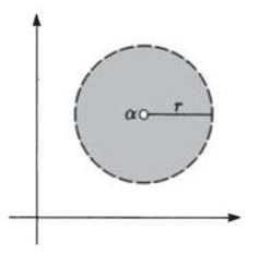
Definition: A function has an isolated singularity at the point if is analytic on a punctured open disc , where , but not at itself.

Note that a function is analytic at a point if it is differentiable on a region containing . Strangely, a function can have a derivative at a point without being analytic there. For example, the function has a derivative at but at no other point, as can easily be verified using the Cauchy-Riemann equations. Therefore this function is not analytic at . Also note with regard to the definition of an isolated singularity that the function MUST be analytic on the whole of the punctured open disc for the singularity to be defined. For example, despite appearances, the function

does not have a singularity at because it is impossible to define a punctured open disc centred at on which is analytic (the function is discontinuous everywhere on the negative real axis, so fails to be analytic there).

I find it appealing that all three types of isolated singularity (removable, poles and essential singularities) can be illustrated by using members of the following family of functions:

where . For example, if we get

which has a removable singularity at . If we get

which has a pole of order at . Finally, if we get

which has an essential singularity at . In each of these three cases, the function is not analytic at but is analytic on a punctured open disc with centre , e.g., or indeed (which can be thought of as a punctured disc with infinite radius). In what follows I will use these three examples to delve into structural definitions of the three types of singularity. I will then explore their classification using Laurent series expansions.

Structural definitions of isolated singularities

Removable singularities

Suppose a function is analytic on the punctured open disc

and has a singularity at . The function has a removable singularity at if there is a function which is analytic at such that

for

We can see that extends the analyticity of to include , so we say that is an analytic extension of to the circle

With removable singularities we always have that exists since

(this will not be true for the other types of singularity) and the name of this singularity comes from the fact that we can effectively `remove’ the singularity by defining .

To apply this to the function

we first observe that the Maclaurin series expansion of is

for

Therefore we can write

for

If we then set

for

we see that extends the analyticity of to include . We also see that

Therefore has a removable singularity at .

Poles of order k, k > 0

Suppose a function is analytic on the punctured open disc

and has a singularity at . The function has a pole of order at if there is a function , analytic at with , such that

for

With poles of order we always have that

as

(which distinguishes them from removable singularities)

and

exists and is nonzero (since ).

To apply this to the function

we first observe that

for

where is the function

for

Since , we see that behaves like near and

as

so the singularity at is not removable. We also see that

Therefore the function has a pole of order at .

Essential singularities

Suppose a function is analytic on the punctured open disc

and has a singularity at . The function has an essential singularity at if the singularity is neither removable nor a pole. Such a singularity cannot be removed in any way, including by mutiplying by any , hence the name.

With essential singularities we have that

does not exist, and does not tend to infinity as .

To apply this to the function

we observe that if we restrict the function to the real axis and consider a sequence of points

then we have that whereas

Therefore

does not exist, so the singularity is not removable, but it is also the case that

so the singularity is not a pole. Since it is neither a removable singularity nor a pole, it must be an essential singularity.

Classification of isolated singularities using Laurent series

By Laurent’s Theorem, a function which is analytic on an open annulus

(shown in the diagram) can be represented as an extended power series of the form

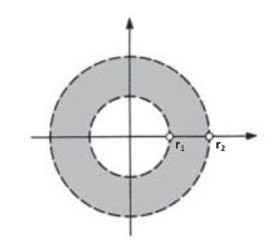
for , which converges at all points in the annulus. It is an `extended’ power series because it involves negative powers of . (The part of the power series involving negative powers is often referred to as the singular part. The part involving non-negative powers is referred to as the analytic part). This extended power series representation is the Laurent series about for the function on the annulus . Laurent series are also often used in the case when is a punctured open disc, in which case we refer to the series as the Laurent series about for the function .

The Laurent series representation of a function on an annulus is unique. We can often use simple procedures, such as finding ordinary Maclaurin or Taylor series expansions, to obtain an extended power series and we can feel safe in the knowledge that the power series thus obtained must be the Laurent series.

Laurent series expansions can be used to classify singularities by virtue of the following result: If a function has a singularity at and if its Laurent series expansion about is

then

(a) has a removable singularity at iff for all ;

(b) has a pole of order at iff for all and ;

(c) has an essential singularity at iff for infinitely many .

To apply this to our three examples, observe that the function

has a singularity at and its Laurent series expansion about is

for . This has no non-zero coefficients in its singular part (i.e., it only has an analytic part) so the singularity is a removable one.

The function

has a singularity at and its Laurent series expansion about is

for . This has for all and , so the singularity in this case is a pole of order .

Finally, the function

has a singularity at and its Laurent series expansion about is

for . This has for infinitely many so the singularity here is an essential singularity.

Singularities in Schwarzschild black holes

One often hears about singularities in the context of black hole physics and I wanted to quickly look at singularities in the particular case of nonrotating black holes. A detailed investigation of the various singularities that appear in exact solutions of Einstein’s field equations was conducted in the 1960s and 1970s by Penrose, Hawking, Geroch and others. There is now a vast literature on this topic. The following discussion is just a quick look at how some ideas involving singularities appear in a simple black hole model.

The spacetime of a nonrotating spherical black hole is usually analysed using the Schwarzschild solution of the Einstein field equations for an isolated spherical mass . In spherical coordinates this is the metric

where

and is the mass of the spherically symmetric static object exterior to which the Schwarzschild metric applies. If we consider only radial motion (i.e., world lines for which ) the Schwarzschild metric simplifies to

We can see that the term in the metric becomes infinite at so there is apparently a singularity here. However, this singularity is `removable’ by re-expressing the metric in a new set of coordinates, and , known as the Eddington-Finkelstein coordinates. The transformed metric has the form

which does not behave badly at . In general relativity, this type of removable singularity is known as a coordinate singularity. Another example is the apparent singularity at the latitude in spherical coordinates, which disappears when a different coordinate system is used.

Since the term in the Schwarzschild metric becomes infinite at , it appears that we also have a singularity at this point. This is not a removable singularity and can in fact be recognised in terms of the earlier discussion above as a pole of order 1 (also called a simple pole).

For teaching purposes, I was trying to find different ways of proving the familiar result that the complex square root function is discontinuous everywhere on the negative real axis. As I was working on alternative proofs, it became very clear to me how sensitive all the proofs were to the particular definition of the principal argument I was using, namely that the principal argument is the unique argument of satisfying . In a sense, this definition manufactures the discontinuity of the complex square root function on the negative real axis, because the principal argument function itself is discontinuous here: the principal argument of a sequence of points approaching the negative real axis from above will tend to , whereas the principal argument of a sequence approaching the same point on the negative real axis from below will tend to . I realised that all the proofs I was coming up with were exploiting this discontinuity of the principal argument function. However, this particular choice of principal argument function is completely arbitrary. An alternative could be to say that the principal argument of is the unique argument satisfying which we can call . The effect of this choice of principal argument function is to make the complex square root function discontinuous everywhere on the positive real axis! It turns out that we can choose an infinite number of different lines to be lines of discontinuity for the complex square root function, simply by choosing different definitions of the principal argument function. The same applies to the complex logarithm function. In this note I want to record some of my thoughts about this.

The reason for having to specify principal argument functions in the first place is that we need to make complex functions of complex variables single-valued rather than multiple-valued, to make them well-behaved with regard to operations like differentiation. Specifying a principal argument function in order to make a particular complex function single-valued is called choosing a branch of the function. If we specify the principal argument function to be where then we define the principal branch of the logarithm function to be

for , and the principal branch of the square root function to be

for with .

If we define the functions and in this way they will be single-valued, but the cost of doing this is that they will not be continuous on the whole of the complex plane (essentially because of the discontinuity of the principal argument function, which both functions `inherit’). They will be discontinuous everywhere on the negative real axis. The negative real axis is known as a branch cut for these functions. Using this terminology, what I want to explore in this short note is the fact that different choices of branch for these functions will result in different branch cuts for them.

To begin with, let’s formally prove the discontinuity of the principal argument function , , and then see how this discontinuity is `inherited’ by the principal logarithm and square root functions. For the purposes of the proof we can consider the sequence of points

where

Clearly, as , we have . However,

whereas

Therefore , so the principal argument function is discontinuous at all points on the negative real axis.

Now consider how the following proof of the discontinuity of on the negative real axis depends crucially on the discontinuity of . We again consider the sequence of points

where

so that . However,

whereas

Therefore , so the principal square root function is discontinuous at all points on the negative real axis.

Now suppose we choose a different branch for the principal logarithm and square root functions, say which as we said earlier satisfies . The effect of this is to change the branch cut of these functions to the positive real axis! The reason is that the principal argument function will now be discontinuous everywhere on the positive real axis, and this discontinuity will again be `inherited’ by the principal logarithm and square root functions.

To prove the discontinuity of the principal argument function on the positive real axis we can consider the sequence of points

where

We have . However,

whereas

Therefore , so the principal argument function is discontinuous at all points on the positive real axis.

We can now again see how the following proof of the discontinuity of on the positive real axis depends crucially on the discontinuity of there. We again consider the sequence of points

where

so that . However,

whereas

Therefore , so the principal square root function is discontinuous at all points on the positive real axis.

There are infinitely many other branches to choose from. In general, if is any real number, we can define the principal argument function to be where

and this will give rise to a branch cut for the principal logarithm and square root functions consisting of a line emanating from the origin and containing all those points such that modulo .

Sir William Rowan Hamilton famously discovered the key rules for quaternion algebra while walking with his wife past a bridge in Dublin in 1843. A plaque now commemorates this event. I needed to use the quaternion rotation operator recently and while digging around the literature on this topic I noticed that a lot of it is quite unclear and over-complicated. A couple of simple, yet vital, ideas, if they were spelt out, would make key results seem less mysterious but these never seem to be mentioned. The vector notation often used in this area also seems to over-complicate things. In this note I want to record some thoughts about the quaternion rotation operator, bringing out some key underlying ideas that (to me) make things seem far less mysterious.

Quaternions are hypercomplex numbers of the form

In many ways (as I will show below) they can usefully be thought about using familiar ideas for two-dimensional complex numbers in which .

In the case of quaternions, the identities discovered by Hamilton determine all possible products of , and . They imply a cyclic relationship when calculating their products (similar to that of the cross products of the three-dimensional basis vectors i, j, k, which is why authors often use these basis vectors when defining quaternions).

Taking products clockwise one obtains

and taking products anticlockwise one obtains

This algebraic structure leads to some interesting differences from the familiar algebra of ordinary two-dimensional complex numbers, particularly non-commutativity of multiplication. Technically, one says that the set of all quaternions with the operations of addition and multiplication constitute a non-commutative division ring, i.e., every non-zero quaternion has an inverse and quaternion products are generally non-commutative.

I was interested to notice that one way in which this algebraic difference with ordinary complex numbers manifests itself is in taking the complex conjugate of products. With ordinary complex numbers and one obtains

since

and therefore

but this is the same as

With the product of two quaternions and we get a different result:

In words, the complex conjugate of the product is the product of the complex conjugates in reverse order. To see this, let

Then

Therefore

But this is the same as

The complex conjugate is used to define the length of a quaternion

as

To find the inverse of a quaternion we observe that

so

For a quaternion

let

A key result that helps to clarify the literature on quaternion rotation is that

This seems mysterious at first but can easily be verified by confirming that when the term on the left hand side is multiplied by itself, the result is :

This result means that any quaternion of the above form can be written as

This is just a familiar two-dimensional complex number! It therefore has an angle associated with it, given by the equations

We can express the quaternion in terms of this angle as

If is a unit quaternion (i.e., ) we then get that

This is the form that is needed in the context of quaternion rotation. It turns out that for any unit quaternion of this form and for any vector the operation

will result in a rotation of the vector through an angle about the vector as the axis of rotation. The direction of rotation is given by the familiar right-hand rule, i.e., the thumb of the right hand points in the direction of the vector and the fingers then curl in the direction of rotation.

As an example, suppose we want to rotate the vector through about the vector in the sense of the right-hand rule.

Looking at the diagram above, we would expect the result to be the vector . Using the quaternion rotation operator to achieve this, we would specify

The resulting vector would be

This result is interpreted as the vector which is exactly what we expected based on the diagram above.

Note that to achieve the same result through conventional matrix algebra we would have to use the rotation matrix

Setting and applying this to the vector we get

This is the same result, but note that this approach is more cumbersome to implement because there are different rotation matrices for different axes of rotation and for different rotation conventions. The above rotation matrix happens to be the one required to achieve a rotation about the y-axis using the right-hand rule. In general, the correct rotation matrix would have to be computed each time to suit the particular rotation required. Once the angle of rotation and the axis of rotation are known, the quaternion rotation operator is easier to specify and implement.

For the purposes of some work I was doing involving ternary numbers, I became interested in finding a quick and easily programmable method for converting prime reciprocals into ternary representation. By trial and error I found a Euclidean-like division algorithm which works well, as illustrated by the following application to the calculation of the ternary representation of the prime reciprocal :

The first equation always has on the left hand side and the remainder in each equation is multiplied by to obtain the left-hand side of the next equation. The procedure halts when a remainder is obtained which is equal to . From then on, the pattern of the coefficients of the prime denominator will repeat indefinitely. In the above example a remainder of is obtained at the sixth step, and the pattern will repeat from then on, so looking at the coefficients of we conclude that the ternary representation of is where the dot notation is used to indicate that the string of digits between the dots repeats indefinitely. This is completely analogous to the fact that the decimal, i.e., base-10, representation of has the repeating cycle structure . Note that the cycle length is in the ternary representation of precisely because is the order of modulo . (The order of an integer modulo a prime is the lowest power of the integer which is congruent to mod . A well known theorem of Fermat guarantees that the order of any integer modulo a prime is at most ).

A further illustration is the computation of the ternary form of , for which the division algorithm yields

before the remainder repeats, giving the ternary representation . The cycle length for is , which is due to the fact that is the order of mod .

In general, for a prime reciprocal , the ternary cycle length will always be the order of mod , and the cycle will repeat from the first digit after the point.

To implement the above algorithm I wrote the following Python program which reads a list of primes from a text file (in this case, the first primes greater than ), then computes the ternary representation of the corresponding prime reciprocals, depositing the output in another text file. The output for each prime reciprocal is the first cycle of ternary digits (the cycle repeats indefinitely thereafter), as well as a statement of the cycle length.

In a series of papers from 1905, his `annus mirabilis’, Albert Einstein analysed Brownian motion and derived the following partial differential equation (known as the diffusion equation) from physical principles to describe the process:

This equation has as a solution the probability density function

(see Einstein, A., 1956, Investigations on the Theory of Brownian Movement, New York: Dover, ISBN 978-0-486-60304-9, pp. 15-16).

Writing this formula can be rewritten as

This is the density of the distribution of the increments of a Wiener process , also commonly referred to as Brownian motion. This continuous-time stochastic process is symmetric about zero, continuous, and has stationary independent increments, i.e., the change from time to time , given by the random variable , has the same probability distribution as the change from time to time , given by the random variable , and the change is also independent of the history of the process before time .

A continuous-time stochastic process which is also symmetric about zero and continuous like the Wiener process, but which has non-stationary increments, has a probability density function of the form

The fact that time appears as a squared term in this formula rather than linearly is enough to destroy the increment-stationarity property of the Wiener process. This can be demonstrated by observing that increment-stationarity requires

and therefore by definition of we must also have

but this not true here since

We have a contradiction and must therefore conclude that

which means that this alternative continuous-time process does not have the increment-stationarity property of the Wiener process. (Note that this kind of contradiction does not arise with the Wiener process: we have which is the same as the distribution of ).

Is there a partial differential equation describing this alternative continuous-time process analogous to the partial differential equation derived by Einstein for the standard Brownian motion process? I did indeed find such a partial differential equation for the alternative process, as follows. Taking partial derivatives of the probability density function

we obtain

Comparing the expressions for and we see that

and this is the required variant of Einstein’s partial differential equation for the alternative continuous-time process.

I was intrigued to find that a slight generalisation of this framework makes it applicable to quantum wave-packet dispersion. To see this, let where and are some parameters. Then the partial differential equation

has as a solution the probability density function

as can be verified by comparing the partial derivatives

and

(As a check, note that all of this reduces to the previously obtained differential equation and probability density function when and ). Now, in quantum mechanics a wave representation of a moving body is obtained as a wave-packet consisting of a superposition of individual plane waves of different wavelengths (or equivalently, different wave numbers ) in the form

where is the Fourier transform of the -space wavefunction at , i.e.,

The wave-packet disperses over time and it has been shown that the probability density as a function of time of such a moving body as the wave-packet disperses, given by , always becomes Gaussian (irrespective of the original shape of the wave-packet) and has the form of the probability density function above, i.e.,

See, for example, Mita, K, 2007, Dispersion of non-Gaussian free particle wave packets, Am. J. Phys. 75 (10), who derives an expression for like the one above with replaced by and

(see equations (15) to (18) on page 952 of the paper). Therefore the partial differential equation

has as a solution the probability density of a moving body undergoing quantum wave-packet dispersion as time progresses (with in the above set-up).