Dr Christian P. H. Salas

Applying Chebyshev’s inequality and the Borel-Cantelli lemma to Brownian motion

Chebyshev’s inequality and the Borel-Cantelli lemma are seemingly disparate results from probability theory but they combine beautifully in demonstrating a curious property of Brownian motion: that it has finite quadratic variation even though it has unbounded linear variation. Not only do the proofs of Chebyshev’s inequality and the Borel-Cantelli lemma have some interesting features themselves, but their application to the variation of Brownian motion also provides a nice example of how to prove explicitly that a sequence of random variables converges almost surely by showing that the probability of the divergence set is zero. In this note I want to bring out this last aspect in particular. (Quick reviews of lim sup, lim inf and the link between almost sure convergence and limp sup are provided in Appendices I and II at the end of this note).

There are two equivalent forms of Chebyshev’s inequality. Letting $X$ denote an integrable random variable with mean $\mu$ and finite non-zero variance $\sigma^2$ , one form of Chebyshev’s inequality says

$P(|X - \mu| \geq k\sigma) \leq \frac{1}{k^2}$

where $k > 0$ is a real number.

Equivalently, if we let $\epsilon = k\sigma$ , then we can write Chebyshev’s inequality as

$P(|X - \mu| \geq \epsilon) \leq \frac{\sigma^2}{\epsilon^2}$

Proof of Chebyshev’s inequality

The following is a proof of the second form. Since $\epsilon > 0$ , we have

$|X - \mu| \geq \epsilon \iff (X - \mu)^2 \geq \epsilon^2$

Let $g(t) = (t - \mu)^2$ so that $\mathbb{E}[g(X)] = \sigma^2$ .

Let

$A = \{\omega : g(X(\omega)) \geq \epsilon^2\}$

$\equiv \{\omega : (X - \mu)^2 \geq \epsilon^2\}$

$\equiv \{\omega : |X - \mu| \geq \epsilon\}$

If $\omega \in A$ then $I_A(\omega) = 1$ and

$\epsilon^2I_A(\omega) \leq g(X(\omega))$

(by definition of $A$ ). However, if $\omega \in A^c$ then $I_A(\omega) = 0$ so it is still true that

$\epsilon^2I_A(\omega) \leq g(X(\omega))$

Thus, this inequality always holds. Taking expectations we get

$\mathbb{E}[\epsilon^2I_A(\omega)] = \epsilon^2P(A) = \epsilon^2P(|X - \mu| \geq \epsilon) \leq \mathbb{E}[g(X(\omega))] = \sigma^2$

Division of both sides by $\epsilon^2$ gives Chebyshev’s inequality.

The Borel-Cantelli lemma actually consists of a pair of results. Let $\{A_k : 1 \leq k\}$ be a sequence of events, i.e., a sequence of subsets of $\Omega$ . Then

$\limsup \limits_{ k } A_k \equiv \bigcap_{n=1}^{\infty} \bigcup_{k=n}^{\infty} A_k$

is the set of all elements $\omega \in \Omega$ that are in an infinity of the subsets $A_k$ . The Borel-Cantelli lemma says the following:

(a) If $\sum_{k=1}^{\infty} P(A_k) < \infty$ then $P\bigg(\limsup \limits_{ k } A_k\bigg) = 0$

(b) If $\{A_k : 1 \leq k\}$ is independent and $\sum_{k=1}^{\infty}P(A_k) = \infty$ then $P\bigg(\limsup \limits_{ k } A_k\bigg) = 1$

Proof of the Borel-Cantelli lemma

(a) For any integer $n \geq 1$ , we can write

$0 \leq P\bigg(\limsup \limits_{ k } A_k\bigg) = P(\bigcap_{n=1}^{\infty} \bigcup_{k=n}^{\infty} A_k) \leq P(\bigcup_{k=n}^{\infty} A_k) \leq \sum_{k=n}^{\infty}P(A_k)$

(the last inequality by subadditivity). Since $\sum_{k=1}^{\infty} P(A_k)$ converges, the tail sums $\sum_{k=n}^{\infty}P(A_k) \rightarrow 0$ as $n \rightarrow \infty$ . Therefore (by a ‘sandwich’ argument) $P\bigg(\limsup \limits_{ k } A_k\bigg) = 0$ .

(b) We have

$\bigg(\limsup \limits_{ k } A_k\bigg)^c = (\bigcap_{n=1}^{\infty} \bigcup_{k=n}^{\infty} A_k)^c$

$= \bigcup_{n=1}^{\infty} (\bigcup_{k=n}^{\infty} A_k)^c = \bigcup_{n=1}^{\infty} \bigcap_{k=n}^{\infty} A_k^c$

$\equiv \bigcup_{n=1}^{\infty} F_n$

(by De Morgan’s laws). Therefore

$1 - P\bigg(\limsup \limits_{ k } A_k\bigg) = P\bigg(\bigg(\limsup \limits_{ k } A_k\bigg)^c\bigg) = P(\bigcup_{n=1}^{\infty} F_n) \leq \sum_{n=1}^{\infty}P(F_n)$

By the product rule for independent events,

$P(F_n) = P(\bigcap_{k=n}^{\infty} A_k^c) = \prod_{k=n}^{\infty}P(A_k^c) = \prod_{k=n}^{\infty}(1 - P(A_k))$

Now, for all $a \geq 0$ we have $1 - a \leq e^{-a}$ . (To see this, let $f(a) = e^{-a} - (1 - a)$ . Then $f(0) = 0$ and for $a > 0$ we have $f^{\prime}(a) = -e^{-a} + 1 > 0$ . Therefore $f(a)$ is an increasing function, so $f(a) \geq f(0)$ for $a \geq 0$ ). It follows that

$1 - P(A_k) \leq \exp(-P(A_k))$

and therefore also

$\prod_{k=n}^{N}(1 - P(A_k)) \leq \exp(-\sum_{k=n}^N P(A_k))$

But $\exp(-\sum_{k=n}^N P(A_k)) \rightarrow 0$ as $N \rightarrow \infty$ . Therefore $P(F_n) = 0$ and $\sum_{n=1}^{\infty}P(F_n) = 0$ , so $1 - P\bigg(\limsup \limits_{ k } A_k\bigg) = 0 \implies P\bigg(\limsup \limits_{ k } A_k\bigg) = 1$ , so the lemma is proved.

To apply these results to the variation of Brownian motion, let

$\triangle_n \equiv \{a = t_0 < t_1 < \cdots < t_n = b\}$

be a partition of the interval $[a, b]$ . Define the mesh of the partition $\triangle_n$ by

$||\triangle_n|| \equiv \max_{1 \leq i \leq n}(t_i - t_{i-1})$

Let us restrict ourselves only to sequences of partitions $\{\triangle_n : 1 \leq n\}$ for which $||\triangle_n|| \rightarrow 0$ , and in particular for which $\sum_{n=1}^{\infty} ||\triangle_n|| < \infty$ . For every $p > 0$ let

$Q_p(f; a, b, \triangle_n) \equiv \sum_{i=1}^{n}|f(t_i) - f(t_{i-1})|^p$

and let

$V_p(f; a, b) \equiv \lim \limits_{||\triangle_n|| \rightarrow 0} Q_p(f; a, b, \triangle_n)$

where $f$ is a real-valued function defined on $[a, b]$ . If $V_p(f; a, b) < \infty$ we will say that $f$ has finite $p^{th}$ variation on $[a, b]$ . In the case $p = 1$ , if $V_1(f; a, b) < \infty$ we will say that $f$ is of bounded linear variation on $[a, b]$ . In the case $p = 2$ , if $V_2(f; a, b) < \infty$ we will say that $f$ is of bounded quadratic variation on $[a, b]$

If we replace $f$ in the above by a Brownian motion $B$ , then we find a curious result: $B$ is of unbounded linear variation almost surely, but it has a finite quadratic variation equal to $b - a$ almost surely. In other words,

$V_1(B; a, b) = \infty$ (a.s.)

$V_2(B; a, b) = b - a$ (a.s.)

We will use Chebyshev’s inequality and the Borel-Cantelli lemma to prove these.

Theorem 1

If $\{\triangle_n : 1 \leq n\}$ is a sequence of partitions of $[a, b]$ with $\sum_{n=1}^{\infty} ||\triangle_n|| < \infty$ (and therefore $||\triangle_n|| \rightarrow 0$ ), then

$Q_2(B; a, b, \triangle_n) = \sum_{i=1}^n |B(t_i) - B(t_{i-1})|^2 \rightarrow b - a$ (a.s.)

as $n \rightarrow \infty$ . In other words, Brownian motion has bounded quadratic variation on $[a, b]$ equal to $b - a$ , almost surely.

Proof:

Observe that, by ‘telescoping’,

$\sum_{i=1}^{n}(t_i - t_{i-1}) = b - a$

Let

$Y_n = \sum_{i=1}^{n}(B(t_i) - B(t_{i-1}))^2 - (b - a)$

$= \sum_{i=1}^{n}\big\{(B(t_i) - B(t_{i-1}))^2 - (t_i - t_{i-1})\big\}$

Note that $\mathbb{E}[Y_n] = 0$ because $\mathbb{E}[(B(t_i) - B(t_{i-1}))^2] = t_i - t_{i-1}$ . Therefore

$\mathbb{V}[Y_n] = \mathbb{E}[Y_n^2]$

$= \mathbb{E}\big[\big(\sum_{i=1}^n \big\{(B(t_i) - B(t_{i-1}))^2 - (t_i - t_{i-1})\big\} \big)^2 \big]$

$= \sum_{i=1}^n \mathbb{E}\big[\big\{(B(t_i) - B(t_{i-1}))^2 - (t_i - t_{i-1})\big\}^2 \big]$

(cross product terms vanish since Brownian motion has independent increments)

$= \sum_{i=1}^n \mathbb{E}\big[(B(t_i) - B(t_{i-1}))^4 - 2(t_i - t_{i-1})(B(t_i) - B(t_{i-1}))^2 + (t_i - t_{i-1})^2 \big]$

$= \sum_{i=1}^n \big(3(t_i - t_{i-1})^2 - 2(t_i - t_{i-1})^2 + (t_i - t_{i-1})^2 \big)$

(since the fourth moment of a zero-mean normal random variable is $3\sigma^4$ and here $\sigma^2 = (t_i - t_{i-1})$ )

$= \sum_{i=1}^n 2(t_i - t_{i-1})^2$

$\leq 2 ||\triangle_n||\sum_{i=1}^n (t_i - t_{i-1})$

$= 2(b - a)||\triangle_n||$

(Since $||\triangle_n|| \rightarrow 0$ , we see already at this stage that $Y_n \rightarrow 0$ in $\mathcal{L}^2$ ).

By the second form of Chebyshev’s inequality we can now write for any $\epsilon > 0$ that

$\sum_{n=1}^{\infty}P(|Y_n| > \epsilon) \leq \sum_{n=1}^{\infty} \frac{\mathbb{E}[Y_n^2]}{\epsilon^2}$

$\leq \frac{2(b - a)}{\epsilon^2}\sum_{n=1}^{\infty}||\triangle_n|| < \infty$

In particular, we can write for any integer $q \geq 1$ that

$\sum_{n=1}^{\infty} P\big(|Y_n| > \frac{1}{q}\big) < \infty$

By the first result in the Borel-Cantelli lemma we can then say

$P\bigg(\limsup \limits_{ k } A_k(q)\bigg) = 0$

where

$A_k(q) = \big\{\omega : |Y_k| > \frac{1}{q}\big\}$

Now,

$\limsup \limits_{ k } A_k(q) = \bigcap_{n=1}^{\infty} \bigcup_{k=n}^{\infty}A_k(q)$

so if $P\bigg(\limsup \limits_{ k } A_k(q)\bigg) = 0$ then we must also have

$P\big(\bigcup_{q=1}^{\infty} \bigcap_{n=1}^{\infty} \bigcup_{k=n}^{\infty}A_k(q)\big) = 0$

But

$\bigcup_{q=1}^{\infty} \bigcap_{n=1}^{\infty} \bigcup_{k=n}^{\infty}A_k(q)$

is the divergence set when considering the almost sure convergence of $Y_n$ to zero. Since the probability of the divergence set is zero, we conclude that $Y_n \rightarrow 0$ a.s., and therefore $Q_p(B; a, b, \triangle_n) \rightarrow b - a$ (a.s.), as required.

Theorem 2

If $\{\triangle_n : 1 \leq n\}$ is a sequence of partitions of $[a, b]$ with $||\triangle_n|| \rightarrow 0$ , then

$Q_1(B; a, b, \triangle_n) = \sum_{i=1}^n |B(t_i) - B(t_{i-1})| \rightarrow \infty$ (a.s.)

as $n \rightarrow \infty$ . In other words, Brownian motion has unbounded linear variation on $[a, b]$ , almost surely.

Proof:

By contradiction. Suppose Brownian motion has bounded linear variation, i.e., $V_1(B; a, b) < \infty$ . Then we can write

$\sum_{i=1}^n |B(t_i) - B(t_{i-1})|^2 \leq \max_{1 \leq i \leq n}|B(t_i) - B(t_{i-1})|\sum_{i=1}^n |B(t_i) - B(t_{i-1})|$

$\leq V_1(B; a, b)\max_{1 \leq i \leq n}|B(t_i) - B(t_{i-1})|$

Since $B$ is uniformly continuous on $[a, b]$ ( $B$ is continuous on $[a, b]$ and any continuous function is uniformly continuous when restricted to a compact set) we can write

$\max_{1 \leq i \leq n}|B(t_i) - B(t_{i-1})| \rightarrow 0$ as $||\triangle_n|| \rightarrow 0$

which if $V_1(B; a, b) < \infty$ implies

$\sum_{i=1}^n |B(t_i) - B(t_{i-1})|^2 \rightarrow 0$ (a.s.)

This contradicts Theorem 1. Therefore $B$ cannot have bounded linear variation and the theorem is proved.

Appendix I Notes on lim sup and lim inf

Let $\{A_k : 1 \leq k \}$ be a sequence of events, i.e., a sequence of subsets of $\Omega$ .

$\limsup \limits_{ k } A_k =$ the set of elements that are in an infinite number of the subsets $A_k$

$\liminf \limits_{ k } A_k =$ the set of elements that are in all but a finite number of the subsets $A_k$

Note that $\liminf \limits_{ k } A_k$ $\subset$ $\limsup \limits_{ k } A_k$ but the inclusion does not go in the opposite direction because $\omega$ can be in an infinity of sets without being in all but a finite number of them, e.g, $\omega$ can be in all odd numbered sets $A_k$ , but not in even numbered ones.

If $\liminf \limits_{ k } A_k = \limsup \limits_{ k } A_k$ we say the sequence has a limit $A = \lim A_k$ .

We can express lim inf and lim sup in terms of unions and intersections of members of the sequence as follows.

$\liminf \limits_{ k } A_k = \bigcup_{n = 1}^{\infty} \bigcap_{k = n}^{\infty} A_k$

$\limsup \limits_{ k } A_k = \bigcap_{n = 1}^{\infty} \bigcup_{k = n}^{\infty} A_k$

To understand the first expression, note that $\omega$ is in all but a finite number of sets if for some $n$ it is in all $A_k$ for $k \geq n$ which we denote $\bigcup_{n=1}^{\infty} \bigcap_{k=n}^{\infty} A_k$ . The $\bigcup_{n=1}^{\infty}$ part means “for some $n$ ” and the $\bigcap_{k=n}^{\infty} A_k$ part means in all $A_k$ for $k \geq n$ .

Similarly, for the second expression, $\omega$ is in an infinity of the sets if for every $n$ it is in some of the $A_k$ for $k \geq n$ which we denote $\bigcap_{n=1}^{\infty} \bigcup_{k=n}^{\infty} A_k$ .

Appendix II Almost sure convergence and its link with lim sup

A sequence of random variables $\{X_n(\omega) : 1 \leq n \}$ is said to converge almost surely to a random variable $X(\omega)$ iff the probability of the divergence set is zero.

The sequence $\{X_n(\omega) : 1 \leq n \}$ fails to converge almost surely to $X(\omega)$ iff for some $k$ and for any $n$ there is some $i \geq n$ such that

$|X_i(\omega) - X(\omega)| \geq \frac{1}{k}$

(so no matter how large I make $n$ , there will always be some $i \geq n$ for which this inequality holds).

Let $E_i(k) = \{\omega : |X_i(\omega) - X(\omega)| \geq \frac{1}{k} \}$ . Then the divergence set is the set of outcomes for which the above divergence condition is true, which we write as

$D = \bigcup_{k = 1}^{\infty} \bigcap_{n=1}^{\infty} \bigcup_{i=n}^{\infty} E_i(k)$

We can also write the divergence set using lim sup as

$D = \bigcup_{k=1}^{\infty} \limsup \limits_{ i } E_i(k)$

A common way to prove almost sure convergence is therefore to prove that

$P(\limsup \limits_{ i } E_i(k) ) = 0$

Brownian motion and fractional Brownian motion as self-similar stochastic processes

The literature involving fractional Brownian motion has expanded over the past three decades or so. Fractional Brownian motion actually has a long history, having been first introduced in the 1940s by the great Andrey Kolmogorov, and then reintroduced and further developed in a seminal paper by Mandelbrot and Van Ness in 1968 (for an interesting personal account of the history of fractional Browninan motion, and further references, see Taqqu, M, 2013, Benoit Mandelbrot and Fractional Browninan Motion, arXiv: 1302.5237v1). The reason for the recent interest is that fractional Brownian motion has a `long memory’ property that standard Brownian motion lacks (unlike standard Brownian motion, fractional Brownian motion does not have independent increments, as will be shown below), making it useful for modelling processes that exhibit long-term persistence of effects. Thus, for example, one finds in the recent literature that the standard Ornstein-Uhlenbeck process with stochastic differential equation

$dX(t) = \theta(\mu - X(t))dt + \sigma dB(t)$

driven by the standard Brownian motion term $dB(t)$ is modified to produce a fractional version with stochastic differential equation

$dX(t) = \theta(\mu - X(t))dt + \sigma dB_H(t)$

driven by the fractional Brownian motion term $dB_H(t)$ with Hurst parameter $\frac{1}{2} < H < 1$ (to be explained below). Similarly, one finds numerous attempts to modify the famous Black-Scholes framework of mathematical finance to incorporate fractional Brownian motion with a view to capturing more long-term memory effects on market movements.

The problem appears to be that stochastic calculus with fractional Brownian motion is much more difficult than with standard Brownian motion, for which we have the well-developed Itô calculus. Itô calculus cannot be used directly with fractional Brownian motion because the long memory property that makes fractional Brownian motion useful in applications also destroys the `semimartingale’ property of standard Brownian motion, which is needed for Itô calculus to work. Numerous attempts have been made in the last two decades to develop a stochastic calculus for fractional Brownian motion which is analogous to Itô’s calculus. This aspect of the literature still seems rather exploratory and fraught with technical difficulties, compared to the Itô calculus framework.

Standard Brownian motion turns out to be a special case of fractional Brownian motion, being characterised by Hurst parameter $H = \frac{1}{2}$ , as will be shown below. Both are self-similar processes (i.e., fractals, or `scale invariant’, or ‘self-affine’ – numerous equivalent terms are used in the literature). In this note I want to clarify for myself some basic aspects of standard Brownian motion and fractional Brownian motion as self-similar stochastic processes.

Mathematical characterisation of self-similarity

To highlight the self-similarity property of Brownian motion which stochastic differential equations capture, it is useful to contrast stochastic differential equations with ordinary differential equations in this regard. The typical solution of a `nice’ ordinary differential equation is a differentiable function like the one shown top left in the figure below.

Such a differentiable function lacks self-similarity because when we `zoom in’ at finer and finer resolutions, as shown in the remaining plates in the figure, we always end up with a straight line. Newtonian calculus is essentially based on this idea – finding the derivative of a smooth curve at a particular point means finding the slope of the straight line that is tangent to the curve at that point. In contrast, the typical solution of a stochastic differential equation driven by Brownian motion is a ‘jumpy’ curve which is actually nowhere differentiable, like the sample path of a standard Brownian motion shown top left in the figure below.

This curve does exhibit self-similarity in the sense that when we zoom in at finer and finer resolutions, as shown in the remaining plates in the figure, we do not get a straight line but rather just an equally ‘jumpy’ Brownian motion. Itô calculus is essentially based on this idea that ‘zooming in’ does not lead to a straight line in the case of Brownian motion, as will be shown when discussing Itô’s formula below.

No matter what scaling we apply in the x-direction, a Brownian motion remains a Brownian motion. This is the idea of self-similarity which is captured mathematically as follows:

Definition 1: A real-valued stochastic process $\{X(t): t \geq 0\}$ is self-similar if there exists a unique $H > 0$ (called a Hurst parameter) such that for any $a > 0$ we have

$\{X(at)\} \,{\buildrel d \over =}\, \{a^HX(t)\}$

(Note that this also implies $X(0) = 0$ , a.s.)

Another key feature that standard Brownian motion and fractional Brownian motion have in common is that their increments are stationary. This can be formally defined as follows:

Definition 2: A stochastic process is said to have stationary increments if the distributions of $\{X(t + h) - X(h)\}$ are independent of $h$ .

It is usual in the literature to refer to a self-similar stochastic process with Hurst parameter H as being H-ss, and one which also has stationary increments as being H-sssi. Both standard Brownian motion and fractional Brownian motion are H-sssi, as will be shown shortly.

Result 1: Let $\{X(t)\}$ be H-sssi, and suppose $\mathbb{E}[X^2(1)] < \infty$ . Then

$\mathbb{E}[X(t)X(s)] = \frac{1}{2}\{t^{2H} + s^{2H} - |t - s|^{2H}\}\mathbb{E}[X^2(1)]$

Proof: Observe that by virtue of the H-ss property we have

$\mathbb{E}[X^2(t)] = \mathbb{E}[X(t)X(t)] = \mathbb{E}[t^H X(1)t^H X(1)] = t^{2H}\mathbb{E}[X^2(1)]$

and due to the additional si property we have

$\mathbb{E}[(X(t) - X(s))^2] = \mathbb{E}[X^2(|t - s|)] = |t - s|^{2H}\mathbb{E}[X^2(1)]$

Therefore

$\mathbb{E}[X(t)X(s)] \equiv \frac{1}{2}\{\mathbb{E}[(X^2(t)] + \mathbb{E}[(X^2(s)] - \mathbb{E}[(X(t) - X(s))^2]\}$

$= \frac{1}{2}\{t^{2H} + s^{2H} - |t - s|^{2H}\}\mathbb{E}[X^2(1)]$

as claimed.

Standard Brownian motion

The key difference between standard Brownian motion and fractional Brownian motion is that the former has independent increments, the latter does not.

Definition 3: A real-valued stochastic process $\{X(t): t \geq 0\}$ is said to have independent increments if for any $m \geq 1$ and for any partition $0 \leq t_0 < t_1 < \cdots < t_m$ , $X(t_1) - X(t_0)$ , . . ., $X(t_m) - X(t_{m-1})$ are independent.

Definition 4: A real-valued stochastic process $\{B(t): t \geq 0\}$ is a standard Brownian motion if it satisfies the following four conditions:
(i) $B(0) = 0$ , a.s.
(ii) it has independent and stationary increments
(iii) for each $t > 0$ , $B(t) \sim N(0, t)$
(iv) its sample paths are continuous, a.s.

Result 2: Standard Brownian motion $B(t)$ is $\frac{1}{2}$ -sssi.

Proof: We need to prove that for any $a > 0$ we have

$\{B(at)\} \,{\buildrel d \over =}\, \{a^{\frac{1}{2}}B(t)\}$

It is actually easier to prove that

$\{a^{-\frac{1}{2}}B(at)\} \,{\buildrel d \over =}\, \{B(t)\}$

which is equivalent. It is obvious by inspection that conditions (i), (ii) and (iv) in Definition 4 apply to $\{a^{-\frac{1}{2}}B(at)\}$ . With regard to (iii), the normality and mean zero of $\{a^{-\frac{1}{2}}B(at)\}$ are obvious by inspection and the variance is

$\mathbb{E}[(a^{-\frac{1}{2}}B(at))^2] = a^{-1} \cdot at = t$

Therefore $\{a^{-\frac{1}{2}}B(at)\} \,{\buildrel d \over =}\, \{B(t)\}$ as required.

Result 3: $\mathbb{E}[B(t)B(s)] = \text{min}\{t, s\}$ .

Proof: Since standard Brownian motion is $\frac{1}{2}$ -sssi, we have by Result 1 that

$\mathbb{E}[B(t)B(s)] = \frac{1}{2}\{t + s - |t - s|\} \equiv \text{min}\{t, s\}$ .

With regard to the martingale property of Brownian motion, we have the following definitions and result.

Definition 5: Let $(\Omega, \mathscr{F}, \mathbb{P})$ be a probability space on which is defined a stochastic process $\{X(t) : t \geq 0\}$ . A filtration for the stochastic process is a collection of $\sigma$ -algebras $\mathbb{F} = \{\mathscr{F}(t) : t \geq 0\}$ satisfying:
(i) $\mathscr{F}(s) \subset \mathscr{F}(t)$ for $0 \leq s < t$
(ii) for each $t \geq 0$ , the stochastic process $X(t)$ at time $t$ is $\mathscr{F}(t)$ -measurable.
$(\Omega, \mathscr{F}, \mathbb{F}, \mathbb{P})$ is then called the filtered probability space for the process.

Intuitively, a filtration at time $t$ is the history of the wanderings of the stochastic process up to that time. Condition (i) says that there is at least as much information in the later $\sigma$ -algebra $\mathscr{F}(t)$ as there is in any earlier $\sigma$ -algebra $\mathscr{F}(s)$ . Condition (ii) says that the information available at time $t$ is always enough to evaluate the stochastic process at that time (a condition known as the ‘adaptivity’ of $X(t)$ to $\mathscr{F}(t)$ ).

Definition 6: A stochastic process $\{X(t) : t \geq 0\}$ is a martingale if it is integrable (i.e., it has a finite expected value at each $t$ ) and for any $s > 0$ we have

$\mathbb{E}[X(t + s) | \mathscr{F}(t)] = X(t)$ , a.s.

where $\mathscr{F}(t)$ is the information about the process up to time $t$ , that is, $\mathbb{F} = \{\mathscr{F}(t) : t \geq 0\}$ is a filtration.

Intuitively, a stochastic process is a martingale if the best guess at time $t$ of its future value is simply its current value at time $t$ . (Note that the martingale property is measure-specific: the stochastic process can be a martingale with respect to a measure $\mathbb{P}$ , while failing to be a martingale with respect to a different measure $\mathbb{Q}$ . It is often possible to ‘convert’ a Brownian-motion-based stochastic process which is not a martingale into a martingale by changing the probability measure appropriately. The conditions for being able to do this are given by a theorem which is well known in mathematical finance, called the Cameron-Martin-Girsanov theorem).

Result 4: Standard Brownian motion $\{B(t)\}$ is a martingale.

Proof: By definition, $B(t) \sim N(0, t)$ , guaranteeing that the process is at all times integrable with $\mathbb{E}[B(t)] = 0$ for all $t$ . Furthermore, for $s < t$ we have

$\mathbb{E}[B(t) | \mathscr{F}(s)] \equiv \mathbb{E}[B(s) | \mathscr{F}(s)] + \mathbb{E}[B(t) - B(s) | \mathscr{F}(s)]$

$= B(s) + \mathbb{E}[B(t) - B(s)]$

$= B(s)$

where the first term in the second equality follows from the fact that $B(s)$ is known for certain when $\mathscr{F}(s)$ is known, and the second term in the second equality follows from the independent increments property of Brownian motion which implies that future increments are independent of all past information.

With regard to stochastic calculus for functions of standard Brownian motion, the key result is Itô’s formula.

Result 5: (Itô’s formula). If $f$ is a deterministic twice continuously differentiable function, then for any $t$ we have

$f(B(t)) = f(B(0)) + \int_0^t f^{\prime}(B(u))dB(u) + \frac{1}{2}\int_0^t f^{\prime \prime}(B(u))du$

or equivalently, in stochastic differential form,

$df(B(t)) = f^{\prime}(B(t))dB(t) + \frac{1}{2}f^{\prime \prime}(B(t))dt$

Proof: (Sketch). An infinitesimal Taylor series expansion of $f(B(t))$ gives

$df(B(t)) = f^{\prime}(B(t))dB(t) + \frac{1}{2}f^{\prime \prime}(B(t))(dB(t))^2 + \frac{1}{3!}f^{\prime \prime \prime}(B(t))(dB(t))^3 + \cdots$

In a Newtonian context (as we saw above when considering the graph of a differentiable function) only the linear term is relevant as we `zoom in’, which in the context of this Taylor expansion would seem to mean that we could discard the terms involving $(dB(t))^2$ , $(dB(t))^3$ , and higher. However, `zooming in’ on the path of a Brownian motion does not lead to a straight line, and in the context of this Taylor expansion that translates into the fact that we can no longer discard the $(dB(t))^2$ term, although we can discard the higher order terms. To see this, suppose we divide the time interval $[0, t]$ into a partition

$\{0, \frac{t}{n}, \frac{2t}{n}, \ldots, \frac{(n-1)t}{n}, t\}$

for some $n > 0$ . Then we have

$\int_0^t (dB(u))^2 = \lim\limits_{n \rightarrow \infty} \sum_{i=1}^n \big(B\big(\frac{ti}{n}\big) - B\big(\frac{t(i-1)}{n}\big)\big)^2 = \lim\limits_{n \rightarrow \infty} \sum_{i=1}^n \big(B\big(\frac{t}{n}\big)\big)^2$

$= \lim\limits_{n \rightarrow \infty} t \sum_{i=1}^n \frac{1}{n}\bigg(\frac{B\big(\frac{t}{n}\big)}{\sqrt{\frac{t}{n}}}\bigg)^2 = t \mathbb{E}[Z^2] = t \mathbb{V}[Z] = t$

where

$Z = \frac{B\big(\frac{t}{n}\big)}{\sqrt{\frac{t}{n}}} \sim N(0, 1)$

The differential form of $\int_0^t (dB(u))^2 = t$ is $(dB(t))^2 = dt$ , which shows that in the case of Brownian motion the $(dB(t))^2$ term cannot be discarded in the above Taylor series expansion because it equals $dt$ , not zero. However, the higher order terms can be discarded because for integers $m > 2$ we get

$\int_0^t (dB(u))^m = \lim\limits_{n \rightarrow \infty} \sum_{i=1}^n \big(B\big(\frac{t}{n}\big)\big)^m = \lim\limits_{n \rightarrow \infty} t^{m/2} \sum_{i=1}^n \frac{1}{n^{(m-2)/2}}\frac{1}{n}\bigg(\frac{B\big(\frac{t}{n}\big)}{\sqrt{\frac{t}{n}}}\bigg)^m$

$= t^{m/2} \bigg(\lim\limits_{n \rightarrow \infty} \frac{1}{n^{(m-2)/2}}\bigg) \cdot(\mathbb{E}[Z^m]) = 0$

Therefore in differential form we have $(dB(t))^m = 0$ for integers $m > 2$ . (Note that now we can also immediately deduce that $dB(t)dt = 0$ from the fact that $(dB(t))^3 = 0$ , since $(dB(t))^3 = (dB(t))^2dB(t) = dtdB(t)$ ). Using these results in the above Taylor series expansion we get the differential form of Itô’s formula.

Itô’s formula greatly facilitates the problem of finding stochastic differential equations for Brownian-motion-based stochastic processes, and also the reverse problem of integrating stochastic differential equations to obtain the corresponding stochastic processes. For example, suppose we modify the standard Brownian motion process by giving it a volatility $\sigma$ , to yield the stochastic process

$X(t) = \sigma B(t)$

and suppose we want to know the stochastic differential equation which the stochastic process $Y(t) = \exp(X(t))$ obeys. Taking the function $f$ in Itô’s formula to be the exponential function and noting that $(d(X(t))^2 = \sigma^2 (dB(t))^2 = \sigma^2 dt$ we get

$dY(t) = f^{\prime}(X(t))dX(t) + \frac{1}{2}f^{\prime \prime}(X(t))(dX(t))^2 = \sigma Y(t) dB(t) + \frac{\sigma^2}{2}Y(t)dt$

As another example, suppose we modify the standard Brownian motion process by giving it a deterministic drift in addition to the volatility $\sigma$ , to yield the stochastic process

$X(t) = \sigma B(t) + \mu t$

and suppose that we again want to know the stochastic differential equation which the stochastic process $Y(t) = \exp(X(t))$ obeys. Taking the function $f$ in Itô’s formula to be the exponential function and noting that

$(d(X(t))^2 = (\sigma dB(t) + \mu dt)^2 = \sigma^2(dB(t))^2 + 2 \sigma \mu dB(t)dt + \mu^2 (dt)^2 = \sigma^2 dt$

we get

$dY(t) = f^{\prime}(X(t))dX(t) + \frac{1}{2}f^{\prime \prime}(X(t))(dX(t))^2$

$= Y(t)(\sigma dB(t) + \mu dt) + \frac{\sigma^2}{2}Y(t)dt$

$= \sigma Y(t) dB(t) + (\mu + \frac{\sigma^2}{2})Y(t)dt$

Fractional Brownian motion

Definition 7: Let $0 < H < 1$ . A mean-zero Gaussian process $\{B_H(t): t \geq 0\}$ is called a fractional Brownian motion with Hurst parameter $H$ if

$\mathbb{E}[B_H(t)B_H(s)] = \frac{1}{2}\{t^{2H} + s^{2H} - |t - s|^{2H}\}\mathbb{E}[B_H^2(1)]$

Note that this covariance structure reduces to that of the standard Brownian motion in Result 3 when $H = \frac{1}{2}$ .

Result 6: Fractional Brownian motion $\{B_H(t): t \geq 0\}$ is H-sssi, but unlike standard Brownian motion, fractional Brownian motion with $H \neq \frac{1}{2}$ does not have independent increments.

Proof: To prove si, simply note that

$\mathbb{E}[(B_H(t) - B_H(s))^2] = \mathbb{E}[B_H^2(t)] + \mathbb{E}[B_H^2(s)] - 2\mathbb{E}[B_H(t)B_H(s)]$

$= |t - s|^{2H}\mathbb{E}[B_H^2(1)]$

Therefore for every $h > 0$ , the two processes $\{B_H(t + h) - B_H(h)\}$ and $\{B_H(t)\}$ have the same distribution. To prove that fractional Brownian motion with $H \neq \frac{1}{2}$ does not have independent increments, define the increments

$\{b_H(j)\} = \{B_H(j+1) - B_H(j)\}$

for integers $j = 0, \pm 1, \ldots$ . The increments $\{b_H(j)\}$ have zero mean, variance

$\mathbb{E}[b_H^2(j)] = \mathbb{E}[(B_H(j+1) - B_H(j))^2] = \mathbb{E}[B_H^2(1)]$

and autocovariance

$\mathbb{E}[b_H(j) b_H(k)]$

$= \mathbb{E}[B_H(j+1)B_H(k+1) - B_H(j+1)B_H(k) - B_H(k+1)B_H(j) + B_H(j)B_H(k)]$

$= \frac{1}{2} \bigg\{|j+1|^{2H} + |k+1|^{2H} - |j - k|^{2H}$

$-|j+1|^{2H} - |k|^{2H} + |j + 1 - k|^{2H}$

$-|k+1|^{2H} - |j|^{2H} + |k + 1 - j|^{2H}$

$+ |j|^{2H} + |k|^{2H} - |j - k|^{2H}\bigg\}\mathbb{E}[B_H^2(1)]$

$= \bigg\{|j - k + 1|^{2H} - 2|j - k|^{2H} + |j - k - 1|^{2H}\bigg\}\mathbb{E}[B_H^2(1)]$

which is nonzero unless $H = \frac{1}{2}$ . (To see that it is zero when $H = \frac{1}{2}$ , suppose without loss of generality that $j > k$ . Then the expression reduces to

$\mathbb{E}[b_H(j) b_H(k)] = \bigg\{(j - k + 1)^{2H} - 2(j - k)^{2H} + (j - k - 1)^{2H}\bigg\}\mathbb{E}[B_H^2(1)]$

which is zero when $H = \frac{1}{2}$ ).

The largest class of stochastic processes to which Itô calculus is applicable is the class of semimartingales, within which martingales (such as Brownian motion) are included. However, fractional Brownian motion with $H \neq \frac{1}{2}$ is not a semimartingale, and therefore not amenable to Itô’s formula. (Clarifying why fractional Brownian motion is not a semimartingale requires the definition of some additional concepts from stochastic analysis which will not be done in this note). However, it is worth noting that fractional Brownian motion does have a stochastic integral representation in terms of standard Brownian motion, as follows.

Result 7: For $0 < H < 1$ and $t > 0$ , fractional Brownian motion $\{B_H(t): t \geq 0\}$ has a stochastic integral representation of the form

$Z(t) = c_H\bigg\{\int_{-\infty}^0 \big((t - u)^{H - \frac{1}{2}} - (-u)^{H - \frac{1}{2}}\big)dB(u) + \int_0^t (t - u)^{H - \frac{1}{2}}dB(u)\bigg\}$

$= c_H\int_{\mathbb{R}} \big(I_{\{u \leq t\}}(t - u)^{H - \frac{1}{2}} - I_{\{u \leq 0\}}(-u)^{H - \frac{1}{2}}\big)dB(u)$

where $c_H$ is a constant.

Proof: Let

$Z(t) = c_H\int_{\mathbb{R}} (I_{\{u \leq t\}}(t - u)^{H - \frac{1}{2}} - I_{\{u \leq 0\}}(-u)^{H - \frac{1}{2}})dB(u)$

Then $Z(t)$ is H-ss. To see this, make the change of variable $u = ts$ . We get

$Z(t) \,{\buildrel d \over =}\, c_H\int_{\mathbb{R}} (I_{\{ts \leq t\}}(t - ts)^{H - \frac{1}{2}} - I_{\{ts \leq 0\}}(-ts)^{H - \frac{1}{2}})dB(ts)$

$\,{\buildrel d \over =}\, t^{H - \frac{1}{2}}c_H\int_{\mathbb{R}} (I_{\{s \leq 1\}}(1 - s)^{H - \frac{1}{2}} - I_{\{s \leq 0\}}(-s)^{H - \frac{1}{2}})t^{\frac{1}{2}}dB(s)$

$\,{\buildrel d \over =}\, t^H c_H\int_{\mathbb{R}} (I_{\{s \leq 1\}}(1 - s)^{H - \frac{1}{2}} - I_{\{s \leq 0\}}(-s)^{H - \frac{1}{2}})dB(s)$

$\,{\buildrel d \over =}\, t^H Z(1)$

(Note that $dB(ts) = t^{\frac{1}{2}}dB(s)$ by Result 2, or we can say $(dB(ts))^2 = d(ts) = tds = (t^{\frac{1}{2}}dB(s))^2$ ). The process $Z(t)$ is also si. To see this, observe that

$\mathbb{E}[(Z(t) - Z(s))^2]$

$= \mathbb{E}\bigg[c_H\int_{\mathbb{R}} [I_{\{u \leq t\}}(t - u)^{H - \frac{1}{2}} - I_{\{u \leq s\}}(s - u)^{H - \frac{1}{2}}]^2du \bigg]$

Making the change of variable $u = s + m$ this becomes

$= \mathbb{E}\bigg[c_H\int_{\mathbb{R}} [I_{\{m \leq t - s\}}((t - s) - m)^{H - \frac{1}{2}} - I_{\{m \leq 0\}}(-m)^{H - \frac{1}{2}}]^2du \bigg]$

$= |t - s|^{2H}\mathbb{E}[Z^2(1)]$

Therefore $Z(t)$ is a H-sssi mean zero Gaussian process and from Result 1 we can conclude that it has the same covariance structure as fractional Brownian motion with Hurst parameter $H$ .

Gauss’s flux theorem for gravity, Poisson’s equation and Newton’s law

Gauss’s flux theorem for gravity (also known as Gauss’s law for gravity) in differential form says that

$\nabla \cdot \mathbf{g} = -4 \pi G \rho$

where $\mathbf{g}$ is the gravitational force, $G$ is the Newtonian gravitational constant and $\rho$ is the (differential) mass density. The link with the scalar potential through $\mathbf{g} = -\nabla \phi$ gives us

$\nabla^2 \phi = 4 \pi G \rho$

(a well known type of partial differential equation known as Poisson’s equation).

In this short note I want to record the observation that one can get quite far towards deriving Gauss’s law for gravity without knowing Newton’s law of universal gravitation, but not all the way. To explore this, suppose that all we know is that the gravitational force depends on mass and radial distance:

$\mathbf{g} = k(M, r) \cdot \mathbf{e_r}$

Here, $k$ is an unspecified function, $M$ is a mass which can be taken as being located at the origin, $r$ is the radial distance from the origin, and $\mathbf{e_r}$ is a radial unit vector.

Now we imagine a closed spherical surface $\delta V$ of radius $r$ centered at the origin. The total flux of the gravitational field $\mathbf{g}$ over the closed surface $\delta V$ is

$\oint_{\delta V} \mathbf{g} \cdot d\mathbf{A} = \oint_{\delta V} k(M, r) \cdot \mathbf{e_r} \cdot d\mathbf{A}$

= $k(M, r) \oint_{\delta V} \mathbf{e_r} \cdot \mathbf{e_r} \cdot dA$

= $k(M, r) \oint_{\delta V} dA$

= $k(M, r) \cdot 4 \pi r^2$

(this explains where the $4 \pi$ comes from).

The total flux is independent of $r$ so to eliminate $r^2$ we must have $k(M, r) = \frac{k^{*}(M)}{r^2}$ where $k^{*}(M)$ is some unspecified function of $M$ , and therefore

$\oint_{\delta V} \mathbf{g} \cdot d\mathbf{A} = k^{*}(M) \cdot 4 \pi$

By the divergence theorem we can write this as

$\oint_{V} \nabla \cdot \mathbf{g} dV = k^{*}(M) \cdot 4 \pi$

and therefore differentiating both sides with respect to $V$ we get

$\nabla \cdot \mathbf{g} = k^{* \prime}(M)\frac{dM}{dV} 4 \pi$

If we set $\frac{dM}{dV} = \rho$ we see that this is nearly Gauss’s law:

$\nabla \cdot \mathbf{g} = k^{* \prime}(M) 4 \pi \rho$

We only need Newton’s law to tell us that $k^{* \prime}(M) = -G$ at this final stage.

Pythagorean triples in a homeomorphism between the 1-sphere and the extended real line

Years ago, I was thinking about various kinds of mappings of prime numbers and wondered in particular what prime numbers would look like when projected from the (extended) real line to the $1$ -sphere by a homeomorphism linking these two spaces. When I did the calculations, I was amazed to find that prime numbers are mapped to a family of Pythagorean triples on the $1$ -sphere. This came as a complete surprise to me at the time, but a quick Google search revealed that that the link between stereographic projection and Pythagorean triples is already well known. Nevertheless, I still find this result interesting and in this note I want to quickly record how I stumbled on it.

Consider the three points $N$ , $Q$ and $P$ in the diagram. Since they are collinear, there must be a scalar $t$ such that

$P = N + t(Q - N)$

Writing this equation in vector form we get

$(x, 0) = (0, 1) + t\big((x_1, x_2) - (0, 1) \big)$

$= (x_1 t, t(x_2 - 1) + 1)$

from which we deduce

$x = x_1 t$

$\implies t = \frac{x}{x_1}$

and

$t(x_2 - 1) + 1 = 0$

$\implies t = \frac{1}{1 - x_2}$

Equating these two expressions for $t$ we get

$\frac{x}{x_1} = \frac{1}{1 - x_2}$

$\implies x = \frac{x_1}{1 - x_2}$

The function $\pi(x_1, x_2) = \frac{x_1}{1 - x_2}$ is the homeomorphism which maps points on the $1$ -sphere to points on the extended real line.

I was more interested in the inverse function $\pi^{-1}(x)$ which maps points on the extended real line to the $1$ -sphere. To find this, observe that

$x^2 + 1 = \frac{x_1^2}{(1 - x_2)^2} + \frac{(1 - x_2)^2}{(1 - x_2)^2}$

Using $x_1^2 + x_2^2 = 1$ we have $x_1^2 = 1 - x_2^2$ so the above equation can be written as

$x^2 + 1 = \frac{1 - x_2^2}{(1 - x_2)^2} + \frac{(1 - 2x_2 + x_2^2)}{(1 - x_2)^2}$

$= \frac{2 - 2x_2}{(1 - x_2)^2} = \frac{2}{1 - x_2}$

Therefore

$x^2 + 1 = \frac{2}{1 - x_2}$

$\implies x_2 = \frac{x^2 - 1}{x^2 + 1}$

and then

$x = \frac{x_1}{1 - x_2}$

$\implies x_1 = \frac{2x}{x^2 + 1}$

Therefore if $x$ is a prime, the corresponding point on the $1$ -sphere is

$\bigg( \frac{2x}{x^2 + 1}, \frac{x^2 - 1}{x^2 + 1} \bigg)$

However, the numbers $2x$ , $x^2 - 1$ and $x^2 + 1$ are then Pythagorean triples, as can easily be demonstrated by showing that these terms satisfy the identity

$(2x)^2 + (x^2 - 1)^2 \equiv (x^2 + 1)^2$

Topological equivalence of the 2-sphere and the extended complex plane (the `Riemann sphere’)

In this short note I want to quickly set out the mathematical details of how the Riemann sphere arises when the point at infinity is added to the complex plane to give the extended complex plane $\Sigma = \mathbb{C}\bigcup \{\infty \}$ , i.e., an explicit homeomorphism which establishes the topological equivalence of the $2$ -sphere and the extended complex plane, giving rise to the name Riemann sphere for the latter.

The $2$ -sphere in $\mathbb{R}^3$ , namely

$S^2 = \{(x_1, x_2, x_3) \in \mathbb{R}^3| x_1^2 + x_2^2 + x_3^2 = 1 \}$

is visualised as sitting in a coordinate system with its centre at the origin, and the complex plane $\mathbb{C}$ is identified with the plane $x_3 = 0$ by identifying $z = x + iy$ , $x, y \in \mathbb{R}$ , with $(x, y, 0)$ for all $z \in \mathbb{C}$ . The point $N = (0, 0, 1)$ is identified as the `north pole’ of $S^2$ , and stereographic projections from $N$ then give rise to a bijective map between $S^2 \backslash \{N \}$ and $\mathbb{C}$ of the form

$\pi: S^2\backslash \{N \} \rightarrow \mathbb{C}$

$\pi: Q \mapsto P$

such that the points $N$ , $Q$ , and $P$ are collinear (but note that we are excluding $N$ from the domain of the bijection at this stage). The situation is illustrated in the following diagram:

To show that $\pi$ is in fact a homeomorphism (i.e., a continuous bijection from $S^2\backslash \{N \}$ to $\mathbb{C}$ whose inverse is also continuous), let $P = (x, y, 0)$ where $z = x + iy \in \mathbb{C}$ , and let

$Q = (x_1, x_2, x_3) \in S^2 \backslash \{N \}$

Since $P$ , $Q$ , and $N$ are collinear, there is some constant $t$ such that

$P = N + t(Q - N)$

Therefore considering the coordinates separately in this equation we have

$\frac{x}{x_1} = t$

$\frac{y}{x_2} = t$

$\frac{1}{1 - x_3} = t$

and so

$x = \frac{x_1}{1-x_3}$

$y = \frac{x_2}{1-x_3}$

Therefore we have

$z = x + iy = \frac{x_1 + ix_2}{1 - x_3}$

and this is the map $\pi: Q \mapsto P$ .

To get the inverse map $\pi^{-1}: P \mapsto Q$ , we observe that

$x^2 + y^2 + 1$

$= \frac{x_1^2}{(1-x_3)^2} + \frac{x_2^2}{(1-x_3)^2} + \frac{(1-x_3)^2}{(1-x_3)^2}$

$= \frac{1 - x_3^2}{(1-x_3)^2} + \frac{1 - 2x_3 + x_3^2}{(1-x_3)^2}$

(using $x_1^2 + x_2^2 + x_3^2 = 1$ )

$= \frac{2 - 2x_3}{(1-x_3)^2}$

$= \frac{2}{1-x_3}$

Therefore $\pi^{-1}: P \mapsto Q$ is given by

$x_1 = x(1-x_3) = \frac{2x}{x^2 + y^2 + 1}$

$x_2 = y(1-x_3) = \frac{2y}{x^2 + y^2 + 1}$

$1 - x_3 = \frac{2}{x^2 + y^2 + 1}$ $\qquad$ $\implies$ $\qquad$ $x_3 = \frac{x^2 + y^2 - 1}{x^2 + y^2 + 1}$

These expressions show that both $\pi$ and $\pi^{-1}$ are continuous, so $\pi$ is a homeomorphism between $S^2\backslash \{N \}$ and $\mathbb{C}$ , i.e., $S^2\backslash \{N \}$ and $\mathbb{C}$ are topologically equivalent.

To complete the picture we need to extend the homeomorphism $\pi$ to include the point $N$ . We do this by defining

$\pi(N) = \infty$

where $\infty$ , known as the point at infinity, is the distinguishing feature that makes the geometry of the present context non-Euclidean (it can be viewed as the point in this geometry where lines which start out parallel eventually meet, something which is impossible in Euclidean geometry). With the addition of the point at infinity into the picture we get the full homeomorphism

$\pi: S^2 \rightarrow \Sigma$

between the $2$ -sphere and the extended complex plane. This explains why the extended complex plane $\Sigma$ is referred to as the Riemann sphere. It is because the extended complex plane is homeomorphic (i.e., topologically equivalent) to the $2$ -sphere in $\mathbb{R}^3$ .

Intuitively, points $Q$ on the $2$ -sphere $S^2$ which are close to the north pole $N$ correspond under $\pi$ to complex numbers $P = z$ with large magnitude $|z|$ , i.e., to complex numbers which are `closer to infinity’ in a sense. Similarly, points $Q^{\prime}$ on the $2$ -sphere which are close to the south pole $S = (0, 0, -1)$ correspond to complex numbers $z^{\prime}$ with small magnitude $|z^{\prime}|$ . Points on the equator of the $2$ -sphere, which intersects the plane $x_3 = 0$ , correspond to the unit circle $|z| = 1$ in the complex plane. The situation is illustrated in the following diagram:

The p-adic number field as a completion of the rationals

In this note I want to explore some of the details involved in the close analogy between:

A). the way Cantor constructed the real number field as the completion of the rationals using Cauchy sequences with the usual Euclidean metric; and

B). the way the p-adic number field can be similarly constructed as the completion of the rationals, but using Cauchy sequences with a different metric (known as an ultrametric).

I have found that exploring this analogy in some detail has allowed me to get quite a good foothold on some of the key features of p-adic analysis.

A basic initial characterisation of p-adic numbers

A lot flows from the basic observation that given a prime number $p$ and a rational number $x = a/b$ , it is always possible to factor out the powers of $p$ in $x$ as in the equation

$x = \frac{a}{b} = p^{n_0}\frac{a_1}{b_1}$

with

$p \nmid a_1b_1$

The exponent $n_0$ , known as the p-adic valuation in the literature, can be negative, zero or positive depending on how the prime $p$ appears (or not) as a factor in the numerator and denominator of the rational number $x = a/b$ .

For example, suppose we specify the prime $p = 7$ . Then we can factor out the powers of $7$ in the rational numbers $56/12$ , $177553$ , and $3/686$ as

$\frac{56}{12} = 7^1 \times \frac{2}{3}$

$177553 = 7^0 \times 177553$

$\frac{3}{686} = 7^{-3} \times \frac{3}{2}$

respectively.

For each prime number $p$ , we can write any positive rational number $x = a/b$ in the power series form

$x = \frac{a}{b} = \sum_{n \ge n_0} a_np^n$

where $n_0$ is the p-adic valuation of $x$ and the coefficients $a_n$ come from the set of least positive residues of $p$ . (These coefficients will always exhibit a repeating pattern in the power series of a rational number). This power series form is called the p-adic expansion of $x$ . In the case $b = 1$ , i.e., when $x$ is a positive integer, the p-adic expansion is just the expansion of $x$ in base $p$ .

If the rational number $x = a/b$ is negative rather than positive, its p-adic expansion can be obtained from the positive version above as

$x = \frac{a}{b} = \sum_{n \ge n_0} b_np^n$

where

$b_{n_0} = p - a_{n_0}$

and

$b_n = (p - 1) - a_n$

for $n > n_0$ .

We can obtain the p-adic expansion for any rational number $x = a/b$ by the following algorithm. Let the p-adic expansion we want to find be

$x = \frac{a}{b} = a_{n_0}p^{n_0} + a_{n_1}p^{n_0+1} + a_{n_2}p^{n_0+2} + \cdots$

$= p^{n_0}(a_{n_0} + a_{n_1}p + a_{n_2}p^2 + a_{n_3}p^3 + \cdots)$

$= p^{n_0}\frac{a_1}{b_1}$

where all fractions are always given in their lowest terms. We deduce that the p-adic expansion of $a_1/b_1$ is then

$\frac{a_1}{b_1} = a_{n_0} + a_{n_1}p + a_{n_2}p^2 + a_{n_3}p^3 + \cdots$

so, since the right hand side equals $a_{n_0}$ mod $p$ , we can compute $a_{n_0}$ as

$a_{n_0} \equiv a_1b_1^{-1}$ (mod $p$ )

Next, we see that

$\frac{a_1}{b_1} - a_{n_0} = a_{n_1}p + a_{n_2}p^2 + a_{n_3}p^3 + \cdots$

$= p(a_{n_1} + a_{n_2}p + a_{n_3}p^2 + a_{n_4}p^3 + \cdots)$

$= p\frac{a_2}{b_2}$

We deduce that the p-adic expansion of $a_2/b_2$ is then

$\frac{a_2}{b_2} = a_{n_1} + a_{n_2}p + a_{n_3}p^2 + a_{n_4}p^3 + \cdots$

so, since the right hand side equals $a_{n_1}$ mod $p$ , we can compute $a_{n_1}$ as

$a_{n_1} \equiv a_2b_2^{-1}$ (mod $p$ )

We continue this process until the repeating pattern in the coefficients is spotted.

For example, suppose we specify the prime to be $p = 5$ and consider the rational number $2/15$ . The p-adic valuation of this rational number is $-1$ since we can write

$\frac{2}{15} = 5^{-1} \cdot \frac{2}{3}$

Therefore we expect the p-adic expansion for $2/15$ to have $p^{-1}$ in its first term. Following the steps of the algorithm we compute the first coefficient as

$a_{n_0} \equiv 2 \times 3^{-1} \equiv 12 \times 3^{-1} \equiv 4$ (mod $5$ )

Then we have

$\frac{2}{3} - 4 = \frac{-10}{3} = 5 \cdot \frac{-2}{3}$

so we can compute the second coefficient as

$a_{n_1} \equiv -2 \times 3^{-1} \equiv 3 \times 3^{-1} \equiv 1$ (mod $5$ )

Then we have

$\frac{-2}{3} - 1 = \frac{-5}{3} = 5 \cdot \frac{-1}{3}$

so we can compute the third coefficient as

$a_{n_2} \equiv -1 \times 3^{-1} \equiv 9 \times 3^{-1} \equiv 3$ (mod $5$ )

Then we have

$\frac{-1}{3} - 3 = \frac{-10}{3} = 5 \cdot \frac{-2}{3}$

so we see immediately that the fourth coefficient will be the same as the second, and the pattern will repeat from this point onwards. Therefore we have obtained the p-adic expansion of $2/15$ as

$\frac{2}{15} = 4p^{-1} + 1 + 3p + p^2 + 3p^3 + p^4 + 3p^5 + \cdots$

It can be shown that the set of all p-adic expansions is an algebraic field. This is called the field of p-adic numbers and is usually denoted by $\mathbb{Q}_p$ in the literature. In the rest of this note I will explore some aspects of the construction of the field $\mathbb{Q}_p$ by analogy with the way Cantor constructed the field of real numbers from the field of rationals. The next section reviews Cantor’s construction of the reals.

Cantor’s construction of the real number field

In Cantor’s construction of the real numbers from the rationals, we regard the latter as a metric space $(\mathbb{Q}, d)$ where the metric $d$ is defined in terms of the ordinary Euclidean absolute value function:

$d(x, y) = \mid x - y \mid$

The central problem in constructing the real number field $\mathbb{R}$ from the field of rationals $\mathbb{Q}$ is that of defining irrational numbers only in terms of rationals. This can be done in alternative ways, e.g., using Dedekind cuts, but Cantor’s approach achieves it using the concept of a Cauchy sequence. A Cauchy sequence in a metric space is a sequence of points which become arbitrarily `close’ to each other with respect to the metric, as we move further and further out in the sequence. More formally, in the context of the metric space $(\mathbb{Q}, d)$ , a sequence $\{q_n \}$ of rationals is a Cauchy sequence if for each $\epsilon > 0$ (where $\epsilon \in \mathbb{Q}$ ) there is an $N \in \mathbb{N}$ such that

$d(q_i, q_j) = \mid q_i - q_j \mid < \epsilon$ for all $i, j \ge N$

For example, if $\epsilon = 10^{-6}$ , then we can be sure that there is a certain point in the Cauchy sequence $\{q_n \}$ beyond which all the terms of the sequence will always be within a millionth of each other in absolute value. If instead we set $\epsilon = 10^{-9}$ , we might have to go further out in the sequence, but we can still be sure that beyond a certain point all the terms of the sequence from then on will be within a billionth of each other in absolute value. And so on.

Cantor’s approach to constructing the reals is based on the idea that any irrational number can be regarded as the limit of Cauchy sequences of rationals, so we can actually define the irrationals as sets of Cauchy sequences of rationals.

To illustrate, consider the irrational number $\sqrt{2}$ . Define three sequences of rationals $\{a_n \}$ , $\{b_n \}$ , $\{x_n \}$ as follows:

$a_0 = 1$

$b_0 = 2$

$x_n = \frac{1}{2}(a_n + b_n)$ for all $n \ge 1$ ,

$a_{n+1} = x_n$ if $x_n^2 < 2$ , otherwise $a_{n+1} = a_n$ ,

$b_{n+1} = b_n$ if $x_n^2 < 2$ , otherwise $b_{n+1} = x_n$ .

For each $n \ge 1$ , $x_n$ lies between $a_n$ and $b_n$ , and at each iteration the closed interval $[a_n, b_n]$ has length

$b_n - a_n = (\frac{1}{2})^n$

(To see this, note that from the definitions of the three sequences above we find that

$b_{n+1} - a_{n+1} = \frac{1}{2}(b_n - a_n)$

so we get the result from this by a simple induction). Also, each closed interval $[a_n, b_n]$ contains $\sqrt{2}$ . Therefore the closed interval $[a_n, b_n]$ is increasingly ‘closing in’ around $\sqrt{2}$ , i.e., we have

$[a_{n+1}, b_{n+1}] \subseteq [a_n, b_n]$

So for each of the sequences $\{a_n \}$ , $\{b_n \}$ , $\{x_n \}$ of rationals, the terms of the sequence are getting closer and closer to each other, and closer to $\sqrt{2}$ . Cantor’s idea was basically to define an irrational such as $\sqrt{2}$ to be the set containing all Cauchy sequences like $\{a_n \}$ , $\{b_n \}$ , and $\{x_n \}$ which converge to that irrational.

Formally, the process involves defining equivalence classes of Cauchy sequences in the metric space $(\mathbb{Q}, d)$ , so that two Cauchy sequences $\{a_n \}$ and $\{b_n \}$ belong to the same equivalence class, denoted $\{a_n \} \thicksim \{b_n \}$ , if for each $\epsilon > 0$ (where $\epsilon \in \mathbb{Q}$ ) there is an $N \in \mathbb{N}$ such that

$d(a_n, b_n) = \mid a_n - b_n \mid < \epsilon$ for all $n \ge N$

It is straightforward to show that $\thicksim$ is an equivalence relation in the sense that it is reflexive (i.e. $\{a_n \} \thicksim \{a_n \}$ for all Cauchy sequences $\{a_n \}$ ), symmetric (i.e., if $\{a_n \} \thicksim \{b_n \}$ then $\{b_n \} \thicksim \{a_n \}$ for all Cauchy sequences $\{a_n \}$ and $\{b_n \}$ ), and transitive (i.e., if $\{a_n \} \thicksim \{b_n \}$ and $\{b_n \} \thicksim \{c_n \}$ then $\{a_n \} \thicksim \{c_n \}$ for all Cauchy sequences $\{a_n \}$ , $\{b_n \}$ and $\{c_n \}$ ).

Cantor defined a real number to be any equivalence class arising from $\thicksim$ , i.e., any set of the form

$\big \{ \{b_n \}: \{b_n \} \thicksim \{a_n \} \big \}$

where $\{a_n \}$ is a Cauchy sequence in the metric space $(\mathbb{Q}, d)$ . Rational numbers are, of course, subsumed in this since any rational number $q$ belongs to the (constant) Cauchy sequence $\{q_n \}$ defined by $q_n = q$ for all $n$ .

It is now possible to define all the standard relations and arithmetic operations on the real numbers constructed in this way, and it can also be shown that the set of reals constructed in this way is isomorphic to the set of reals defined by alternative means, such as Dedekind cuts.

The set of reals constructed in this way can be regarded as the completion of the set of rationals in the sense that it is obtained by adding to the set of rationals all the limits of all possible Cauchy sequences in $(\mathbb{Q}, d)$ which are irrational. In general, a metric space is said to be complete if every Cauchy sequence in that metric space converges to a point within that metric space. Clearly, therefore, the metric space $(\mathbb{Q}, d)$ is not complete since, for example, we found Cauchy sequences of rationals above which converge to $\sqrt{2} \notin \mathbb{Q}$ . However, it is a basic result of elementary real analysis that the metric space $(\mathbb{R}, d)$ is complete. It is also a basic result that the completion of a field gives another field, so since $\mathbb{Q}$ is a field it must also be the case that $\mathbb{R}$ is a field.

Archimedian vs. non-archimedian absolute values and ultrametric spaces

In constructing the p-adic number field it becomes important to distinguish between two types of absolute value function on a field, namely archimedian and non-archimedian absolute values. All absolute values on a field by definition have the properties that they assign the value 0 only to the field element 0, they assign the positive value $\mid x \mid$ to each non-zero field element $x$ , and they satisfy $\mid xy \mid = \mid x \mid \mid y \mid$ and the usual triangle inequality

$\mid x + y \mid \le \mid x \mid + \mid y \mid$

The usual Euclidean absolute value function used above on $\mathbb{Q}$ , of course, satisfies these conditions, and is called archimedian because it has the property that there is no limit to the size of the absolute values that can be assigned to integers. We can write this as

sup $\{\mid n \mid : n \in \mathbb{Z} \} = +\infty$

Non-archimedian absolute values do not have this property. In addition to the basic conditions that all absolute values must satisfy, non-archimedian absolute values must also satisfy the additional condition

$\mid x + y \mid \le max \{\mid x \mid, \mid y \mid \}$

which is known as the ultrametric triangle inequality. It is obviously the case that the usual Euclidean absolute value function used above on $\mathbb{Q}$ (an archimedian absolute value function) does not satisfy this ultrametric triangle inequality condition, e.g.,

$\mid 1 + 1 \mid \nleq max \{\mid 1 \mid, \mid 1 \mid \}$

In fact, it follows from the ultrametric triangle inequality condition that non-archimedian absolute values of integers can never exceed $1$ , because if the condition is to hold for the absolute value function then we can write for any integer $n$ :

$\mid n + 1 \mid \leq max \{\mid n \mid, 1 \}$

and so by induction we must have

$\mid n^2 \mid \leq max \{ \mid n \mid, 1 \}$

Then if $\mid n \mid \geq 1$ we would have $\mid n^2 \mid \leq \mid n \mid$ which implies $\mid n \mid \leq 1$ , and so $\mid n \mid = 1$ in this case. It is not possible for $\mid n \mid$ to exceed $1$ , so in the case of non-archimedian absolute values we have

sup $\{\mid n \mid : n \in \mathbb{Z} \} = 1$

Any absolute value function which does not satisfy the above ultrametric triangle inequality condition is called archimedian, and these are the only two possible types of absolute values. To see that these are the only two possible types, suppose we have an absolute value function such that

sup $\{\mid n \mid : n \in \mathbb{Z} \} = C$

where $C > 1$ . Then there must exist an integer $m$ whose absolute value exceeds $1$ , and so $\mid m^k \mid = \mid m \mid^k$ gets arbitrarily large as $k$ grows, so $C$ cannot be finite. The absolute value function must be archimedian in this case. Otherwise, we must have $C \leq 1$ , but since for all absolute values it must be the case that $\mid 1 \mid = 1$ , it must be the case that $C = 1$ if $C$ is finite. Thus we must have a non-archimedian absolute value in this case and there are no other possibilities.

The trick in constructing the p-adic number field from the rationals is to use a certain non-archimedian absolute value function satisfying the ultrametric triangle inequality condition to define the metric over $\mathbb{Q}$ , rather than the usual (archimedian) Euclidean absolute value function. In this regard we have the following:

Theorem 1. Define a metric on a field by $d(x, y) = \mid x - y \mid$ . Then the absolute value function in this definition is non-archimedian if and only if for all field elements $x$ , $y$ , $z$ we have

$d(x, y) \le max \{d(x, z), d(z, y) \}$

Proof: Suppose first that the absolute value function is non-archimedian. Applying it to the equation

$(x - y) = (x - z) + (z - y)$

gives

$d(x, y) \le max \{d(x, z), d(z, y) \}$

Conversely, suppose the given metric inequality holds. Then setting $y = -w$ and $z = 0$ in the metric inequality we get

$d(x, -w) \le max \{d(x, 0), d(0, -w) \}$

which is equivalent to

$\mid x + w \mid \leq max \{\mid x \mid, \mid w \mid \}$

thus proving that the absolute value function is non-archimedian.

A metric for which the inequality in Theorem 1 is true is called an ultrametric, and a space endowed with an ultrametric is called an ultrametric space. Such spaces have curious properties which have been studied extensively. In some ways, however, using a non-archimedian absolute value makes analysis much easier than in the usual archimedian case. In this regard we have the following result pertaining to Cauchy sequences with respect to a non-archimedian absolute value function, which is NOT true for archimedian absolute values:

Theorem 2. A sequence $\{x_n \}$ of rational numbers is a Cauchy sequence with respect to a non-archimedian absolute value if and only if we have

$\lim_{n \rightarrow \infty} \mid x_{n+1} - x_n \mid = 0$

Proof: Letting $m = n + r > n$ , we have

$\mid x_m - x_n \mid = \mid x_{n+r} - x_{n+r-1} + x_{n+r-1} - x_{n+r-2} + \cdots + x_{n+1} - x_n \mid$

$\leq max \{\mid x_{n+r} - x_{n+r-1} \mid, \mid x_{n+r-1} - x_{n+r-2} \mid, \dots, \mid x_{n+1} - x_n \mid \}$

$= \mid x_{n+1} - x_n \mid$

because the absolute value is non-archimedian. We then have that if $\{x_n \}$ is Cauchy then the terms get arbitrarily closer as $n \rightarrow \infty$ so we must have $\lim_{n \rightarrow \infty} \mid x_{n+1} - x_n \mid = 0$ . Conversely, if $\lim_{n \rightarrow \infty} \mid x_{n+1} - x_n \mid = 0$ is true, then we must also have $\lim_{n \rightarrow \infty} \mid x_m - x_n \mid = 0$ for any $m > n$ , so the conditions of a Cauchy sequence are satisfied.

It is important to note that Theorem 2 is false for archimedian absolute values. The classic counterexample involves the partial sums of the harmonic series (which is divergent in terms of Euclidean absolute values). Consider the following three partial sums in particular:

$x_n = 1 + \frac{1}{2} + \cdots \frac{1}{n}$

$x_{n+1} = 1 + \frac{1}{2} + \cdots \frac{1}{n} + \frac{1}{n+1}$

$x_{2n} = 1 + \frac{1}{2} + \cdots \frac{1}{n} + \frac{1}{n+1} + \frac{1}{n+2} + \cdots + \frac{1}{2n}$

Then we have

$\lim_{n \rightarrow \infty} \mid x_{n+1} - x_n \mid = \lim_{n \rightarrow \infty} \frac{1}{n+1} = 0$

so the condition of Theorem 2 is satisfied. However,

$\mid x_{2n} - x_n \mid = \frac{1}{n+1} + \frac{1}{n+2} + \cdots + \frac{1}{2n}$

$\geq \frac{1}{2n} + \frac{1}{2n} + \cdots + \frac{1}{2n}$

$= \frac{n}{2n} = \frac{1}{2}$

Therefore it is not true in this case that $\lim_{n \rightarrow \infty} \mid x_m - x_n \mid = 0$ for any $m > n$ , so the conditions of a Cauchy sequence are not satisfied here. It is only in the context of non-archimedian absolute values that this works.

Constructing the p-adic number field as the completion of the rationals

To obtain the p-adic number field as the completion of the field of rationals in a way analogous to how Cantor obtained the reals from the rationals, we use an ultrametric based on a non-archimedian absolute value known as the p-adic absolute value.

For each prime $p$ there is an associated p-adic absolute value on $\mathbb{Q}$ obtained by factoring out the powers of $p$ in any given rational $q \in \mathbb{Q}$ to get

$q = p^{n_0}\frac{a}{b}$

with

$p \nmid ab$

With this factorisation in hand, the p-adic absolute value of $q$ is then defined as

$\mid q \mid_p = p^{-n_0}$

if $q \neq 0$ , and we set $\mid 0 \mid_p = 0$ . (As mentioned earlier, the number $n_0$ is called the p-adic valuation of $q$ ).

It is straightforward to verify that this is a non-archimedian absolute value on $\mathbb{Q}$ . It has some surprising features. For example, unlike the usual Euclidean absolute value function on $\mathbb{Q}$ which can take any non-negative value on a continuum, the p-adic absolute value function can only take values in the discrete set

$\{p^{-n_0} : n_0 \in \mathbb{Z} \} \cup {0}$

For example, in the case of the $7$ -adic absolute value we have

$\mid 35 \mid_7 = \mid 7 \times 5 \mid_7 = \frac{1}{7}$

$\mid \frac{56}{12} \mid_7 = \mid 7 \times \frac{2}{3} \mid_7 = \frac{1}{7}$

$\mid 177553 \mid_7 = \mid 7^0 \times 177553 \mid_7 = 1$

$\mid \frac{3}{686} \mid_7 = \mid 7^{-3} \times \frac{3}{2} \mid_7 = 7^3 = 343$

Note that the $7$ -adic absolute value of $3/686$ is large, while that of $35$ is small.

Now consider the metric space $(\mathbb{Q}, d_p)$ where $d_p$ is defined as

$d_p(x, y) = \mid x - y \mid_p$

By virtue of Theorem 1, $d_p$ is an ultrametric and $(\mathbb{Q}, d_p)$ is an ultrametric space. Since the p-adic absolute value function has some counterintuitive features, it is not surprising that $d_p$ also gives some counterintuitive results. For example, the numbers $1627$ and $2$ are much `closer’ to each other with regard to this ultrametric than the numbers $3$ and $2$ , because

$d_p(1627, 2) = \mid 1627 - 2 \mid_p = \mid 1625 \mid_p = \mid 5^3 \times 13\mid_p = \frac{1}{125}$

whereas

$d_p(3, 2) = \mid 3 - 2 \mid_p = \mid 1 \mid_p = 1$

In addition, we can use it to show that the sequence $\{x_n \}$ where

$x_n = 1 + p + p^2 + p^3 + \cdots + p^n$

is Cauchy with respect to $d_p$ , whereas it is violently non-Cauchy with respect to the usual Euclidean absolute value. We have

$\lim_{n \rightarrow \infty} \mid x_{n+1} - x_n \mid_p = \lim_{n \rightarrow \infty} \mid p^{n+1}\mid_p = \lim_{n \rightarrow \infty}p^{-(n+1)} = 0$

It follows from Theorem 2 in the previous section that the sequence $\{x_n \}$ is Cauchy with respect to the p-adic absolute value. In fact, the infinite series

$x_n = 1 + p + p^2 + p^3 + \cdots$

has the sum $\frac{1}{1-p}$ in the ultrametric space $(\mathbb{Q}, d_p)$ (this formula can be derived in the usual way for geometric series) but its sum is undefined in $(\mathbb{Q}, d)$ .

The following Theorem proves that the ultrametic space $(\mathbb{Q}, d_p)$ is not complete in a way which is analogous to how $(\mathbb{Q}, d)$ is not complete.

Theorem 3. The field $\mathbb{Q}$ of rational numbers is not complete with respect to the p-adic absolute value.

Proof: To prove this, we will create a Cauchy sequence with respect to the p-adic absolute value function whose limit does not belong to $\mathbb{Q}$ .

Let $1 < a \leq p-1$ be an integer. Recall that a property of the Euler totient function is that for any prime $p$ and any integer $n \geq 1$ we have

$\phi(p^{n+1}) = p^n(p - 1)$

Also recall the Euler-Fermat Theorem which says that if $gcd(a, m) = 1$ then

$a^{\phi(m)} \equiv 1$ (mod $m$ )

With these in hand, consider the sequence ${x_n} = {a^{p^n}}$ . Then since we have $gcd(a, p^{n+1}) = 1$ , the Euler-Fermat Theorem tells us that

$a^{p^n(p-1)} \equiv 1$ (mod $p^{n+1}$ )

Therefore

$x_{n+1} - x_n = a^{p^{n+1}} - a^{p^n} = a^{p^n}(a^{p^n(p-1)} - 1)$

must be divisible by $p^n$ , so we have

$\mid x_{n+1} - x_n \mid_p \leq p^{-n}$

and so the sequence ${x_n} = {a^{p^n}}$ is Cauchy with respect to the p-adic absolute value, by virtue of Theorem 2. If we call the limit of this sequence

$x = \lim_{n \rightarrow \infty} x_n$

we can write the following:

$\lim_{n \rightarrow \infty} x_{n+1} = \lim_{n \rightarrow \infty} x_n$

$\lim_{n \rightarrow \infty} a^{p^{n+1}} = \lim_{n \rightarrow \infty} a^{p^n}$

$\lim_{n \rightarrow \infty} (a^{p^n})^p = \lim_{n \rightarrow \infty} a^{p^n}$

$(\lim_{n \rightarrow \infty} a^{p^n})^p = \lim_{n \rightarrow \infty} a^{p^n}$

$x^p = x$

$x^{p-1} = 1$

Therefore since $a \neq 1$ , the limit of the sequence must be a nontrivial $(p-1)$ -th root of unity, so it cannot belong to $\mathbb{Q}$ . This proves that the ultrametric space $(\mathbb{Q}, d_p)$ is not complete.

Although $\mathbb{Q}$ is not complete with regard to the p-adic absolute value, we can construct the p-adic completion $\mathbb{Q}_p$ in a manner analogous to Cantor’s construction of $\mathbb{R}$ as a completion of $\mathbb{Q}$ . Investigating the fine details of this and the properties of $\mathbb{Q}_p$ then lead one into the rich literature on p-adic analysis, which I hope to explore further in future notes.

Maple code for quantum scattering from an Eckart potential

One of the more complicated-looking Schrödinger wavefunctions arises from a scattering (i.e., positive energy) problem involving an Eckart potential. These wavefunctions are expressed in terms of Gauss hypergeometric functions and as part of some numerical work I was doing using Maple software I wanted to see how easy or difficult it would be to write a Maple procedure that would compute and plot these objects. It turned out to be not too difficult and I want to record this Maple code in the present note. The following diagram illustrates the basic setup for scattering from an Eckart potential that will be considered here.

The Eckart potential was first introduced in 1930 (Eckart, C, 1930, The penetration of a potential barrier by electrons, Phys Rev 35, Issue 11, pp. 1303-1309) and has the form

$V(x) = \frac{V_0}{\cosh^2\big(\frac{x}{a}\big)}$

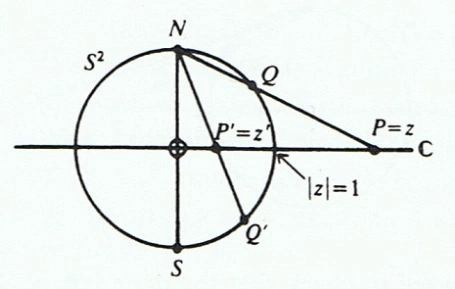
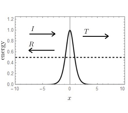
where $V_0$ is the height of the potential at the origin and $a$ is its width. We assume that a travelling wave of predetermined amplitude $I$ is moving from left to right towards the origin, corresponding to a free particle of mass $m$ and energy $E$ , where $0 < E < V_0$ . The particle is scattered in the region around the origin where the potential is nonzero, being reflected with probability $R$ and transmitted (by quantum tunnelling, since $E < V_0$ ) with probability $T$ . 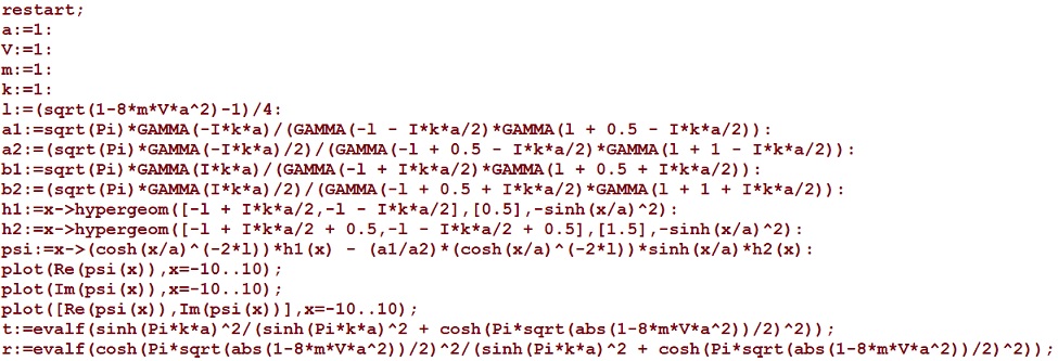Usually, the main focus in scattering problems is on the calculation of $R$ (called the reflection coefficient) and $T$ (called the transmission coefficient) for different energy levels.

The time-independent Schrödinger equation for scattering from an Eckart potential of this form can be written as

$-\frac{\hbar^2}{2m} \frac{d^2\psi}{dx^2} + \bigg[\frac{V_0}{\cosh^2\big(\frac{x}{a}\big)} - E\bigg]\psi = 0$

To rescale this for numerical work we can divide through by $-\frac{\hbar^2}{m}$ to get

$\frac{1}{2} \frac{d^2\psi}{dx^2} + [E^{\prime} - V^{\prime}]\psi = 0$

where

$E^{\prime} = \frac{mE}{\hbar^2}$

and

$V^{\prime} = \frac{mV_0}{\hbar^2 \cosh^2\big(\frac{x}{a}\big)}$

To obtain $E^{\prime}$ explicitly, we observe that far away from the origin the potential is zero, so the above equation reduces to

$\frac{d^2\psi}{dx^2} + 2E^{\prime}\psi = 0$

This is a second-order linear ordinary differential equation with a travelling wave solution of the general form

$\psi = Ae^{i\sqrt{2E^{\prime}}x} + Be^{-i\sqrt{2E^{\prime}}x}$

where $k = \sqrt{2E^{\prime}}$ is the wavenumber. We are free to assign any positive value we like to the wavenumber $k$ in scattering problems. This choice of $k$ will then determine $E^{\prime}$ and $E$ . To begin with, we will set $k = 1$ here, which implies $E^{\prime} = \frac{1}{2}$ .

To obtain $V^{\prime}$ explicitly, we note that we are able to assign any value we like to $V_0$ and $a$ so, to begin with, we will choose $V_0 = \frac{\hbar}{m}$ and $a = 1$ to give us the rescaled potential

$V^{\prime} = \frac{1}{\cosh^2(x)}$

which is of unit height and width. This is the setup shown in the diagram above. Therefore the scattering equation we will be implementing to begin with is

$\frac{1}{2} \frac{d^2\psi}{dx^2} + \bigg[\frac{1}{2} - \frac{1}{\cosh^2(x)}\bigg]\psi = 0$

This quantum system can be solved exactly in terms of Gauss hypergeometric functions of the form ${}_2F_1\big([\alpha, \beta], [\gamma], z\big)$ , i.e., with two upper parameters, $\alpha$ and $\beta$ , and one lower parameter, $\gamma$ . (For details, see ter Haar, D, 1975, Problems in quantum mechanics, London: Pion, Chapter 1, Problem 14, Chapter 2, Problem 8, and also Blinder, S, 2011, Scattering by a Symmetrical Eckart Potential, Wolfram Demonstrations Project). Here we will focus on adapting the (rather complicated) exact solution to the case specified above. Given the four parameters $a$ , $V_0$ , $m$ and $k = \frac{\sqrt{2mE}}{\hbar}$ , let

$\lambda = \frac{1}{4}\bigg[\sqrt{1 - \frac{8mV_0a^2}{\hbar^2}} - 1\bigg]$

$a_1 = \frac{\sqrt{\pi}\cdot \Gamma(-ika)}{\Gamma\big(-\lambda - \frac{ika}{2}\big) \cdot \Gamma\big(\lambda + \frac{1}{2} - \frac{ika}{2}\big)}$

$a_2 = \frac{\sqrt{\pi}\cdot \Gamma(-ika)/2}{\Gamma\big(-\lambda + \frac{1}{2} - \frac{ika}{2}\big) \cdot \Gamma\big(\lambda + 1 - \frac{ika}{2}\big)}$

Then the exact solution of the general time-independent Schrödinger equation for this problem is the wavefunction

$\psi = \bigg[\cosh^2\bigg(\frac{x}{a}\bigg)\bigg]^{-2\lambda}\cdot{}_2F_1\bigg(\bigg[-\lambda+\frac{ika}{2}, -\lambda - \frac{ika}{2}\bigg], \bigg[\frac{1}{2}\bigg], -\sinh^2\bigg(\frac{x}{a}\bigg)\bigg)$

$-\frac{a_1}{a_2} \bigg[\cosh\bigg(\frac{x}{a}\bigg)\bigg]^{-2\lambda} \cdot \sinh\bigg(\frac{x}{a}\bigg)\cdot{}_2F_1\bigg(\bigg[-\lambda+\frac{ika}{2}+\frac{1}{2}, -\lambda - \frac{ika}{2}+\frac{1}{2}\bigg], \bigg[\frac{3}{2}\bigg], -\sinh^2\bigg(\frac{x}{a}\bigg)\bigg)$

The exact solution for our particular specifications is then obtained by setting $a = 1$ , $V_0 = 1$ , $m = 1$ and $k = 1$ in this wavefunction. This solution has both real and imaginary parts which are plotted together in the diagram below.

The reflection and transmission coefficients for this scattering problem are given by the formulas

$R = \frac{\cosh^2\bigg(\frac{\pi}{2}\cdot\sqrt{\big|1 - \frac{8mV_0a^2}{\hbar^2}\big|}\bigg)}{\sinh^2(\pi k a)+\cosh^2\bigg(\frac{\pi}{2}\cdot\sqrt{\big|1 - \frac{8mV_0a^2}{\hbar^2}\big|}\bigg)}$

$T = \frac{\sinh^2(\pi k a)}{\sinh^2(\pi k a)+\cosh^2\bigg(\frac{\pi}{2}\cdot\sqrt{\big|1 - \frac{8mV_0a^2}{\hbar^2}\big|}\bigg)}$

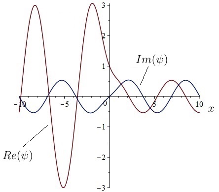
Evaluating these with $a = 1$ , $V_0 = 1$ , $m = 1$ , $k = 1$ and $\hbar = 1$ we get a probability of reflection $R = 0.88$ and a probability of transmission $T = 0.12$ .

I produced the above wavefunction plot, and calculated the corresponding reflection and transmission probabilities, using the following Maple code:

Wavefunction plots and reflection and transmission probabilities for different Eckart scattering parameters can now easily be obtained by simply varying the parameters $a$ , $V$ , $m$ and $k$ in the above code.

Overview of Sturm-Liouville theory: the maths behind quantum mechanics

Sturm-Liouville theory was developed in the 19th century in the context of solving differential equations. When one studies it in depth for the first time, however, one experiences a sudden realisation that this is the mathematics providing the basic framework for quantum mechanics. In quantum mechanics we envisage a quantum state (a time-dependent function) expressed as a superposition of eigenfunctions of a self-adjoint operator (usually referred to as a Hermitian operator) representing an observable. The coefficients of the eigenfunctions in this superposition are probability amplitudes. A measurement of the observable quantity represented by the Hermitian operator produces one of the eigenvalues of the operator with a probability proportional to the square of the modulus of the eigenfunction corresponding to that eigenvalue in the superposition. It is the fact that the operator is self-adjoint that ensures the eigenvalues are real (and thus observable), and furthermore, that the eigenfunctions corresponding to the eigenvalues form a complete and orthogonal set of functions enabling quantum states to be represented as a superposition in the first place (i.e., an eigenfunction expansion akin to a Fourier series). The Sturm-Liouville theory of the 19th century has essentially this same structure and in fact Sturm-Liouville eigenvalue problems are important more generally in mathematical physics precisely because they frequently arise in attempting to solve commonly-encountered partial differential equations (e.g., Poisson’s equation, the diffusion equation, the wave equation, etc.), particularly when the method of separation of variables is employed.

The present note provides an overview of the key ideas in Sturm-Liouville theory and I will begin by considering a nice discussion of a vibrating string problem in Courant & Hilbert’s classic text, Methods of Mathematical Physics (Volume I). Although the problem is simple and the treatment in Courant & Hilbert a bit terse, it (remarkably) brings up a lot of the key features of Sturm-Liouville theory which apply more generally in a wide variety of physics problems. I will then consider Sturm-Liouville theory in a more general setting, emphasising the role of the Sturm-Liouville differential operator.

On page 287 of Volume I, Courant & Hilbert write the following:

Equation (12) here is the one-dimensional wave equation

$\frac{\partial^2 u}{\partial x^2} = \mu^2 \frac{\partial^2 u}{\partial t^2}$

which (as usual) the authors are going to solve by using a separation of variables of the form

$u(x, t) = v(x) g(t)$

As Courant & Hilbert explain, the problem then involves finding the function $v(x)$ by solving the second-order homogeneous linear differential equation

$\frac{\partial^2 v}{\partial x^2} + \lambda v = 0$

subject to the boundary conditions

$v(0) = v(\pi) = 0$

Although not explicitly mentioned by Courant & Hilbert at this stage, equations (13) and (13a) in fact constitute a full blown Sturm-Liouville eigenvalue problem. Despite being very simple, this setup captures many of the typical features encountered in a wide variety of such problems in physics. It is instructive to explore the text underneath equation (13a):

Not all these requirements can be fulfilled for arbitrary values of the constant $\lambda$ … the boundary conditions can be fulfilled if and only if $\lambda = n^2$ is the square of an integer $n$ .

To clarify this, we can try to solve (13) and (13a) for the three possible cases: $\lambda < 0$ , $\lambda = 0$ and $\lambda > 0$ . Suppose first that $\lambda < 0$ . Then $-\lambda > 0$ and the auxiliary equation for (13) is

$D^2 = - \lambda$

$\implies$

$D = \pm \sqrt{- \lambda}$

Thus, we can write the general solution of (13) in this case as

$v = \alpha e^{\sqrt{-\lambda} x} + \beta e^{-\sqrt{-\lambda} x} = A \mathrm{cosh} \big(\sqrt{-\lambda} x\big) + B \mathrm{sinh} \big(\sqrt{-\lambda} x\big)$

where $A$ and $B$ are constants to be determined from the boundary conditions. From the boundary condition $v(0) = 0$ we conclude that $A = 0$ so the equation reduces to

$v = B \mathrm{sinh} \big(\sqrt{-\lambda} x\big)$

But from the boundary condition $v(\pi) = 0$ we are forced to conclude that $B = 0$ since $\mathrm{sinh} \big(\sqrt{-\lambda} \pi\big) \neq 0$ . Therefore there is only the trivial solution $v(x) = 0$ in the case $\lambda < 0$ .

Next, suppose that $\lambda = 0$ . Then equation (13) reduces to

$\frac{\mathrm{d}^2 v}{\mathrm{d} x^2} = 0$

$\implies$

$v = A + Bx$

From the boundary condition $v(0) = 0$ we must conclude that $A = 0$ , and the boundary condition $v(\pi) = 0$ means we are also forced to conclude that $B = 0$ . Thus, again, there is only the trivial solution $v(x) = 0$ in the case $\lambda = 0$ .

We see that nontrivial solutions can only be obtained when $\lambda > 0$ . In this case we have $-\lambda < 0$ and the auxiliary equation is

$D^2 = - \lambda$

$\implies$

$D = \pm i \sqrt{\lambda}$

Thus, we can write the general solution of (13) in this case as

$v = \alpha e^{i \sqrt{\lambda} x} + \beta e^{- i \sqrt{\lambda} x} = A \mathrm{cos} \big(\sqrt{\lambda} x\big) + B \mathrm{sin} \big(\sqrt{\lambda} x\big)$

where $A$ and $B$ are again to be determined from the boundary conditions. From the boundary condition $v(0) = 0$ we conclude that $A = 0$ so the equation reduces to

$v = B \mathrm{sin} \big(\sqrt{\lambda} x\big)$

But from the boundary condition $v(\pi) = 0$ we must conclude that, if $B \neq 0$ , then we must have $\sqrt{\lambda} = n$ where $n = 1, 2, 3, \ldots$ . Thus, we find that for each $n = 1, 2, 3, \ldots$ , the eigenvalues of this Sturm-Liouville problem are $\lambda_n = n^2$ , and the corresponding eigenfunctions are $v = B \mathrm{sin}\big(n x\big)$ . The coefficient $B$ is undetermined and must be specified through some normalisation process, for example by setting the integral of $v^2$ between $0$ and $\pi$ equal to $1$ and then finding the value of $B$ that is consistent with this. In Courant & Hilbert they have (implicitly) simply set $B = 1$ .

Some features of this solution are typical of Sturm-Liouville eigenvalue problems in physics more generally. For example, the eigenvalues are real (rather than complex) numbers, there is a minimum eigenvalue ( $\lambda_1 = 1$ ) but not a maximum one, and for each eigenvalue there is a unique eigenfunction (up to a multiplicative constant). Also, importantly, the eigenfunctions here form a complete and orthogonal set of functions. Orthogonality refers to the fact that the integral of a product of any two distinct eigenfunctions over the interval $(0, \pi)$ is zero, i.e.,

$\int_0^{\pi} \mathrm{sin}(nx) \mathrm{sin}(mx) \mathrm{d} x = 0$

for $n \neq m$ , as can easily be demonstrated in the same way as in the theory of Fourier series. Completeness refers to the fact that over the interval $(0, \pi)$ the infinite set of functions $\mathrm{sin} (nx)$ , $n = 1, 2, 3, \ldots$ , can be used to represent any sufficiently well behaved function $f(x)$ using a Fourier series of the form

$f(x) = \sum_{n=1}^{\infty} a_n \mathrm{sin} (nx)$

All of this is alluded to (without explicit explanation at this stage) in the subsequent part of this section of Courant & Hilbert’s text, where they go on to provide the general solution of the vibrating string problem. They write the following:

The properties of completeness and orthogonality of the eigenfunctions are again a typical feature of the solutions of Sturm-Liouville eigenvalue problems more generally, and this is one of the main reasons why Sturm-Liouville theory is so important to the solution of physical problems involving differential equations. To get a better understanding of this, it is helpful to develop Sturm-Liouville theory in a more general setting by starting with a standard second-order homogeneous linear differential equation of the form

$\alpha(x) \frac{\mathrm{d}^2 y}{\mathrm{d} x^2} + \beta(x) \frac{\mathrm{d} y}{\mathrm{d} x} + \gamma(x) y = 0$

where the variable $x$ is confined to an interval $a \leq x \leq b$ .

Let

$p(x) = \mathrm{exp} \bigg(\int \mathrm{d} x \frac{\beta(x)}{\alpha(x)}\bigg)$

$q(x) = \frac{\gamma(x)}{\alpha(x)} p(x)$

Dividing the differential equation by $\alpha(x)$ and multiplying through by $p(x)$ we get

$p(x) \frac{\mathrm{d}^2 y}{\mathrm{d} x^2} + \frac{\beta(x)}{\alpha(x)} p(x) \frac{\mathrm{d} y}{\mathrm{d} x} + \frac{\gamma(x)}{\alpha(x)} p(x) y = 0$

$\iff$

$\frac{\mathrm{d}}{\mathrm{d} x} \bigg(p(x) \frac{\mathrm{d} y}{\mathrm{d} x} \bigg) + q(x) y = 0$

$\iff$

$L y = 0$

where

$L = \frac{\mathrm{d}}{\mathrm{d} x} \bigg(p(x) \frac{\mathrm{d} }{\mathrm{d} x} \bigg) + q(x)$

is called the Sturm-Liouville differential operator. Thus, we see already that a wide variety of second-order differential equations encountered in physics will be able to be put into a form involving the operator $L$ , so results concerning the properties of $L$ will have wide applicability.

Using the Sturm-Liouville operator we can now write the defining differential equation of Sturm-Liouville theory in an eigenvalue-eigenfunction format that is very reminiscent of the setup in quantum mechanics outlined at the start of this note. The defining differential equation is

$L \phi = - \lambda w \phi$

where $w(x)$ is a real-valued positive weight function and $\lambda$ is an eigenvalue corresponding to the eigenfunction $\phi$ . This differential equation is often written out in full as

$\frac{\mathrm{d}}{\mathrm{d} x} \bigg(p(x) \frac{\mathrm{d} \phi}{\mathrm{d} x} \bigg) + \big(q(x) + \lambda w(x)\big) \phi = 0$

with $x \in [a, b]$ . In Sturm-Liouville problems, the functions $p(x)$ , $q(x)$ and $w(x)$ are specified at the start and, crucially, the function $\phi$ is required to satisfy particular boundary conditions at $a$ and $b$ . The boundary conditions are a key aspect of each Sturm-Liouville problem; for a given form of the differential equation, different boundary conditions can produce very different problems. Solving a Sturm-Liouville problem involves finding the values of $\lambda$ for which there exist non-trivial solutions of the defining differential equation above subject to the specified boundary conditions. The vibrating string problem in Courant & Hilbert (discussed above) is a simple example. We obtain the differential equation (13) in that problem by setting $p(x) = 1$ , $q(x) = 0$ and $w(x) = 1$ in the defining Sturm-Liouville differential equation.

We would now like to prove that the eigenvalues in a Sturm-Liouville problem will always be real and that the eigenfunctions will form an orthogonal set of functions, as claimed earlier. To do this, we need to consider a few more developments. In Sturm-Liouville theory we can apply $L$ to both real and complex functions, and a key role is played by the concept of the inner product of such functions. Using the notation $f(x)^{*}$ to denote the complex conjugate of the function $f(x)$ , we define the inner product of two functions $f$ and $g$ over the interval $a \leq x \leq b$ as

$(f, g) = \int_a^b \mathrm{d} x f(x)^{*} g(x)$

and we define the weighted inner product as

$(f, g)_w = \int_a^b \mathrm{d} x w(x) f(x)^{*} g(x)$

where $w(x)$ is the real-valued positive weight function mentioned earlier. A key result in the theory is Lagrange’s identity, which says that for any two complex-valued functions of a real variable $u(x)$ and $v(x)$ , we have

$v(Lu)^{*} - u^{*} Lv = \frac{\mathrm{d}}{\mathrm{d} x} \bigg[p(x) \bigg(v \frac{\mathrm{d}u^{*}}{\mathrm{d}x} - u^{*}\frac{\mathrm{d}v}{\mathrm{d}x}\bigg) \bigg]$

This follows from the form of $L$ , since

$v(Lu)^{*} - u^{*} Lv$

$= v\bigg[\frac{\mathrm{d}}{\mathrm{d} x} \bigg(p(x) \frac{\mathrm{d}u^{*}}{\mathrm{d} x} \bigg) + q(x) u^{*}\bigg] - u^{*} \bigg[\frac{\mathrm{d}}{\mathrm{d} x} \bigg(p(x) \frac{\mathrm{d} v}{\mathrm{d} x} \bigg) + q(x) v\bigg]$

$= v \frac{\mathrm{d}}{\mathrm{d} x} \bigg(p(x) \frac{\mathrm{d}u^{*}}{\mathrm{d} x} \bigg) - u^{*} \frac{\mathrm{d}}{\mathrm{d} x} \bigg(p(x) \frac{\mathrm{d} v}{\mathrm{d} x} \bigg)$

$= v \frac{\mathrm{d}}{\mathrm{d} x} \bigg(p(x) \frac{\mathrm{d}u^{*}}{\mathrm{d} x} \bigg) + \frac{\mathrm{d} v}{\mathrm{d} x} \bigg(p(x) \frac{\mathrm{d}u^{*}}{\mathrm{d} x} \bigg) - u^{*} \frac{\mathrm{d}}{\mathrm{d} x} \bigg(p(x) \frac{\mathrm{d} v}{\mathrm{d} x} \bigg) - \frac{\mathrm{d} u^{*}}{\mathrm{d} x} \bigg(p(x) \frac{\mathrm{d} v}{\mathrm{d} x} \bigg)$

$= \frac{\mathrm{d}}{\mathrm{d} x} \bigg(p(x) v \frac{\mathrm{d}u^{*}}{\mathrm{d} x} \bigg) - \frac{\mathrm{d}}{\mathrm{d} x} \bigg(p(x) u^{*} \frac{\mathrm{d} v}{\mathrm{d} x} \bigg)$

$= \frac{\mathrm{d}}{\mathrm{d} x} \bigg[p(x) \bigg(v \frac{\mathrm{d}u^{*}}{\mathrm{d}x} - u^{*}\frac{\mathrm{d}v}{\mathrm{d}x}\bigg) \bigg]$

Using the inner product notation, we can write Lagrange’s identity in an alternative form that reveals the crucial role played by the boundary conditions in a Sturm-Liouville problem. We have

$(Lu, v) - (u, Lv) = \int_a^b (Lu)^{*} v \mathrm{d} x - \int_a^b u^{*} Lv \mathrm{d} x$

$= \int_a^b \frac{\mathrm{d}}{\mathrm{d} x} \bigg[p(x) \bigg(v \frac{\mathrm{d}u^{*}}{\mathrm{d}x} - u^{*}\frac{\mathrm{d}v}{\mathrm{d}x}\bigg) \bigg] \mathrm{d} x$

$= \int_a^b \mathrm{d} \bigg[p(x) \bigg(v \frac{\mathrm{d}u^{*}}{\mathrm{d}x} - u^{*}\frac{\mathrm{d}v}{\mathrm{d}x}\bigg) \bigg]$

$= \bigg[p(x) \bigg(v \frac{\mathrm{d}u^{*}}{\mathrm{d}x} - u^{*}\frac{\mathrm{d}v}{\mathrm{d}x}\bigg) \bigg]_a^b$

For some boundary conditions the final term here is zero and then we will have

$(Lu, v) = (u, Lv)$

When this happens, the operator in conjunction with the boundary conditions is said to be self-adjoint. As an example, a so-called regular Sturm-Liouville problem involves solving the differential equation

$\frac{\mathrm{d}}{\mathrm{d} x} \bigg(p(x) \frac{\mathrm{d} \phi}{\mathrm{d} x} \bigg) + \big(q(x) + \lambda w(x)\big) \phi = 0$

subject to what are called separated boundary conditions, taking the form

$A_1 \phi(a) + A_2 \phi^{\prime}(a) = 0$

and

$B_1 \phi(b) + B_2 \phi^{\prime}(b) = 0$

In this case, the operator $L$ is self-adjoint. To see this, suppose the functions $u$ and $v$ satisfy these boundary conditions. Then at $a$ we have

$A_1 u(a)^{*} + A_2 u^{\prime}(a)^{*} = 0$

and

$A_1 v(a) + A_2 v^{\prime}(a) = 0$

from which we can deduce that

$\frac{u^{\prime}(a)^{*}}{u(a)^{*}} = -\frac{A_1}{A_2} = \frac{v^{\prime}(a)}{v(a)}$

$\implies$

$v(a) u^{\prime}(a)^{*} = u(a)^{*} v^{\prime}(a)$

Similarly, at the boundary point $b$ we find that

$v(b) u^{\prime}(b)^{*} = u(b)^{*} v^{\prime}(b)$

These results then imply

$\bigg[p(x) \bigg(v \frac{\mathrm{d}u^{*}}{\mathrm{d}x} - u^{*}\frac{\mathrm{d}v}{\mathrm{d}x}\bigg) \bigg]_a^b = 0$

so the operator $L$ is self-adjoint as claimed. As another example, a singular Sturm-Liouville problem involves solving the same differential equation as in the regular problem, but subject to the boundary condition that $p(x)$ is zero at either $a$ or $b$ or both, while being positive for $a < x < b$ . If $p(x)$ does not vanish at one of the boundary points, then $\phi$ is required to satisfy the same boundary condition at that point as in the regular problem. Clearly we will have

$\bigg[p(x) \bigg(v \frac{\mathrm{d}u^{*}}{\mathrm{d}x} - u^{*}\frac{\mathrm{d}v}{\mathrm{d}x}\bigg) \bigg]_a^b = 0$

in this case too, so the operator $L$ will also be self-adjoint in the case of a singular Sturm-Liouville problem. As a final example, suppose the Sturm-Liouville problem involves solving the same differential equation as before, but with periodic boundary conditions of the form

$\phi(a) = \phi(b)$

$\phi^{\prime}(a) = \phi^{\prime}(b)$

and

$p(a) = p(b)$

Then if $u$ and $v$ are two functions satisfying these boundary conditions we will have

$\bigg[p(x) \bigg(v \frac{\mathrm{d}u^{*}}{\mathrm{d}x} - u^{*}\frac{\mathrm{d}v}{\mathrm{d}x}\bigg) \bigg]_a^b$

$= p(b) \bigg(v(b) u^{\prime}(b)^{*} - u(b)^{*} v^{\prime}(b)\bigg) - p(a) \bigg(v(a) u^{\prime}(a)^{*} - u(a)^{*} v^{\prime}(a)\bigg)$

$= p(a) \bigg[\bigg(v(b) u^{\prime}(b)^{*} - v(a) u^{\prime}(a)^{*}\bigg) + \bigg(u(a)^{*} v^{\prime}(a) - u(b)^{*} v^{\prime}(b)\bigg)\bigg] = 0$

So again, the operator $L$ will be self-adjoint in the case of periodic boundary conditions. Note, for example, that the singular and periodic cases arise when attempting to solve Schrödinger’s equation for the hydrogen atom.

The key reason for focusing so much on the self-adjoint property of the operator $L$ is that the eigenvalues of a self-adjoint operator are always real, and the eigenfunctions are orthogonal. Note that by orthogonality of the eigenfunctions in the more general context we mean that

$(\phi_n, \phi_m)_w = \int_a^b \mathrm{d} x w(x) \phi_n(x)^{*} \phi_m(x) = 0$

whenever $\phi_n(x)$ and $\phi_m(x)$ are eigenfunctions corresponding to two distinct eigenvalues.

To prove that the eigenvalues are always real, suppose that $\phi(x)$ is an eigenfunction corresponding to an eigenvalue $\lambda$ . Then we have

$L \phi = - \lambda w \phi$

and so

$(L \phi, \phi) = (- \lambda w \phi, \phi) = \int_a^b (- \lambda w \phi)^{*} \phi \mathrm{d} x = -\lambda^{*} \int_a^b (w \phi)^{*} \phi \mathrm{d} x$

$= -\lambda^{*}\int_a^b \mathrm{d}x w(x)|\phi(x)|^2$

But we also have

$(\phi, L \phi) = (\phi, - \lambda w \phi) = \int_a^b \phi^{*}(- \lambda w \phi) \mathrm{d} x = -\lambda \int_a^b \phi^{*} (w \phi) \mathrm{d} x$

$= -\lambda\int_a^b \mathrm{d}x w(x)|\phi(x)|^2$

Therefore if the operator is self-adjoint we can write

$(L \phi, \phi) - (\phi, L \phi) = (\lambda - \lambda^{*}) \int_a^b \mathrm{d}x w(x)|\phi(x)|^2 = 0$

$\implies$

$\lambda = \lambda^{*}$

since $\int_a^b \mathrm{d}x w(x)|\phi(x)|^2 > 0$ , so the eigenvalues must be real. In particular, this must be the case for regular and singular Sturm-Liouville problems, and for Sturm-Liouville problems involving periodic boundary conditions.

To prove that the eigenfunctions are orthogonal, let $\phi(x)$ and $\psi(x)$ denote two eigenfunctions corresponding to distinct eigenvalues $\lambda$ and $\mu$ respectively. Then we have

$L \phi = - \lambda w \phi$

$L \psi = - \mu w \psi$

and so by the self-adjoint property we can write

$(L \phi, \psi) - (\phi, L \psi) = \int_a^b (- \lambda w \phi)^{*} \psi \mathrm{d} x - \int_a^b \phi^{*} (- \mu w \psi) \mathrm{d} x$

$= (\mu - \lambda) \int_a^b \mathrm{d}x w(x)\phi(x)^{*} \psi(x) = 0$

Since the eigenvalues are distinct, the only way this can happen is if

$(\phi, \psi)_w = \int_a^b \mathrm{d}x w(x)\phi(x)^{*} \psi(x) = 0$

so the eigenfunctions must be orthogonal as claimed.

In addition to being orthogonal, the eigenfunctions $\phi_n(x)$ , $n = 1, 2, 3, \dots$ , of a Sturm-Liouville problem with specified boundary conditions also form a complete set of functions (I will not prove this here), which means that any sufficiently well-behaved function $f(x)$ for which $\int_a^b\mathrm{d} x |f(x)|^2$ exists can be represented by a Fourier series of the form

$f(x) = \sum_{n=1}^{\infty} a_n \phi_n(x)$

for $x \in [a, b]$ , where the coefficients $a_n$ are given by the formula

$a_n = \frac{(\phi_n, f)_w}{(\phi_n, \phi_n)_w} = \frac{\int_a^b \mathrm{d}x w(x) \phi_n(x)^{*} f(x)}{\int_a^b \mathrm{d}x w(x) |\phi_n(x)|^2}$

It is the completeness and orthogonality of the eigenfunctions that makes Sturm-Liouville theory so useful in solving linear differential equations, because (for example) it means that the solutions of many second-order inhomogeneous linear differential equations of the form

$\frac{\mathrm{d}}{\mathrm{d} x} \bigg(p(x) \frac{\mathrm{d} \phi}{\mathrm{d} x} \bigg) + q(x) \phi = F(x)$

with suitable boundary conditions can be expressed as a linear combination of the eigenfunctions of the corresponding Sturm-Liouville problem

$\frac{\mathrm{d}}{\mathrm{d} x} \bigg(p(x) \frac{\mathrm{d} \phi}{\mathrm{d} x} \bigg) + \big(q(x) + \lambda w(x)\big) \phi = 0$

with the same boundary conditions. To illustrate this, suppose this Sturm-Liouville problem with boundary conditions $\phi(a) = \phi(b) = 0$ has an infinite set of eigenvalues $\lambda_k$ and corresponding eigenfunctions $\phi_k(x)$ , $k = 1, 2, 3, \dots$ , which are orthogonal and form a complete set. We will assume that the solution of the inhomogeneous differential equation above is an infinite series of the form

$\phi(x) = \sum_{k = 1}^{\infty} a_k \phi_k(x)$

where the coefficients $a_k$ are constants, and we will find these coefficients using the orthogonality of the eigenfunctions. Since for each $k$ it is true that

$\frac{\mathrm{d}}{\mathrm{d} x} \bigg(p \frac{\mathrm{d} \phi_k}{\mathrm{d} x} \bigg) + q \phi_k = - \lambda_k w(x) \phi_k$

we can write

$\frac{\mathrm{d}}{\mathrm{d} x} \bigg(p \frac{\mathrm{d} \phi}{\mathrm{d} x} \bigg) + q \phi$

$= \frac{\mathrm{d}}{\mathrm{d} x} \bigg(p \sum_{k = 1}^{\infty} a_k \frac{\mathrm{d} \phi_k}{\mathrm{d} x} \bigg) + q \sum_{k=1}^{\infty} a_k \phi_k$

$= \sum_{k=1}^{\infty} a_k \bigg[\frac{\mathrm{d}}{\mathrm{d} x} \bigg(p \frac{\mathrm{d} \phi_k}{\mathrm{d} x} \bigg) + q \phi_k\bigg]$

$= \sum_{k=1}^{\infty} a_k\big[- \lambda_k w(x) \phi_k\big]$

$= - \sum_{k=1}^{\infty} a_k \lambda_k w(x) \phi_k$

Thus, in the inhomogeneous equation

$\frac{\mathrm{d}}{\mathrm{d} x} \bigg(p(x) \frac{\mathrm{d} \phi}{\mathrm{d} x} \bigg) + q(x) \phi = F(x)$

we can put

$F(u) = - \sum_{k=1}^{\infty} a_k \lambda_k w(u) \phi_k(u)$

To find the $m$ th coefficient $a_m$ we can multiply both sides by $\phi_m(u)^{*}$ and integrate. By orthogonality, all the terms in the sum on the right will vanish except the one involving $\phi_m(u)$ . We will get

$\int_a^b \phi_m(u)^{*} F(u) \mathrm{d}u = - \int_a^b a_m \lambda_m w(x) \phi_m(u)^{*}\phi_m(u) \mathrm{d} u$

$= -a_m \lambda_m (\phi_m, \phi_m)_w$

$\implies$

$a_m = -\int_a^b \frac{\phi_m(u)^{*} F(u)}{\lambda_m (\phi_m, \phi_m)_w}\mathrm{d} u$

Having found a formula for the coefficients $a_k$ , we can now write the solution of the original inhomogeneous differential equation as

$\phi(x) = \sum_{k = 1}^{\infty} a_k \phi_k(x)$

$= \sum_{k = 1}^{\infty} \bigg(-\int_a^b \frac{\phi_k(u)^{*} F(u)}{\lambda_k (\phi_k, \phi_k)_w}\mathrm{d} u\bigg) \phi_k(x)$

$= \int_a^b \mathrm{d} u \bigg(-\sum_{k = 1}^{\infty} \frac{\phi_k(u)^{*} \phi_k(x)}{\lambda_k (\phi_k, \phi_k)_w}\bigg) F(u)$

$= \int_a^b \mathrm{d} u G(x, u) F(u)$

where

$G(x, u) \equiv -\sum_{k = 1}^{\infty} \frac{\phi_k(u)^{*} \phi_k(x)}{\lambda_k (\phi_k, \phi_k)_w}$

is the eigenfunction expansion of the Green’s function for the inhomogeneous problem above.