Ornstein-Uhlenbeck process: derivation and simulation of its pdf and moments

The Ornstein-Uhlenbeck process is widely used in the stochastic modelling of mean-reverting processes. In the present note, I want to record a derivation I produced for a lecture of the pdf and moments of an Ornstein-Uhlenbeck process exhibiting mean-reversion to zero with a stochastic differential equation (SDE) of the form

$dx = -\gamma x dt + \sigma dW \quad \quad \quad \quad (1)$

where $\gamma$ and $\sigma$ are constants and $W(t)$ is a standard Wiener process. I used the Euler–Maruyama method with a time step of $dt = 0.01$ in Python to generate and plot a sample path of this process from $t = 0$ up to $t = 10$ , setting the initial position as $x(0) = 0.6$ and the values $\gamma = 0.5$ and $\sigma = 0.3$ . The following picture shows this sample path:

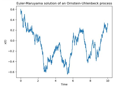
The mean-reversion to zero is clear from the plot and arises due to the $-\gamma$ parameter in the drift term of the SDE, which tends to pull the process back down when $x(t)$ goes above zero and back up when $x(t)$ goes below zero.

The Fokker-Planck equation of the SDE in (1) is easily obtained as

$\frac{\partial \rho(x, t)}{\partial t} = \gamma \frac{\partial}{\partial x} [x \rho(x, t)] + \frac{\sigma^2}{2}\frac{\partial^2 \rho(x, t)}{\partial x^2} \quad \quad \quad (2)$

and this can be used to derive a stationary pdf for the Ornstein-Uhlenbeck process corresponding to a long-term equilibrium situation in which the pdf is not time-varying, so $\partial \rho/\partial t = 0$ . From (2) we then get

$0 = \gamma \frac{\partial}{\partial x} [x \rho(x, t)] + \frac{\sigma^2}{2}\frac{\partial^2 \rho(x, t)}{\partial x^2}$

$= \frac{d}{d x} \bigg[\gamma x \rho(x) + \frac{\sigma^2}{2} \frac{d \rho(x)}{dx} \bigg] \quad \quad \quad \quad (3)$

Equation (3) tells us that the sum of the two terms in the square brackets must be equal to a constant. Setting this constant equal to zero gives us

$\frac{\sigma^2}{2} \frac{d \rho(x)}{dx} = - \gamma x \rho(x)$

and so

$\frac{d \rho(x)/dx}{\rho} = -\frac{2 \gamma x}{\sigma^2}$

from which we deduce the form of the stationary pdf to be

$\rho(x) = N \exp\big(-\frac{\gamma x^2}{\sigma^2}\big)$

We can find an expression for $N$ from the normalisation condition

$N \int_{-\infty}^{\infty} \exp\big(-\frac{\gamma x^2}{\sigma^2}\big) dx = 1 \quad \quad \quad \quad (4)$

Making the change of variable $y = \sqrt{\gamma} x/ \sigma$ we can rewrite (4) as

$N \frac{\sigma}{\sqrt{\gamma}} \int_{-\infty}^{\infty} \exp(-y^2) = 1$

from which we get

$N = \frac{\sqrt{\gamma}}{\sigma I_0} \quad \quad \quad \quad (5)$

where

$I_0 = \int_{-\infty}^{\infty} \exp(-y^2)dy \quad \quad \quad \quad (6)$

The moments of the Ornstein-Uhlenbeck process are obtained as

$\langle x^n \rangle = \int_{-\infty}^{\infty} x^n \rho(x) dx = N \int_{-\infty}^{\infty} x^n \exp\big(-\frac{\gamma x^2}{\sigma^2}\big) dx \quad \quad \quad \quad (7)$

Making the change of variable $y = (\sqrt{\gamma}/\sigma)x$ , we have $x^n = (\sigma/\sqrt{\gamma})^n y^n$ and $dx = (\sigma /\sqrt{\gamma})dy$ . Using these substitutions together with the expression for $N$ in (5) above we get

$\langle x^n \rangle = \frac{\sqrt{\gamma}}{\sigma I_0} \int_{-\infty}^{\infty} \frac{\sigma^{n+1}}{(\sqrt{\gamma})^{n+1}}y^n \exp(-y^2)dy = \frac{\sigma^n}{(\sqrt{\gamma})^n} \frac{I_n}{I_0} \quad \quad \quad \quad (8)$

where

$I_n = \int_{-\infty}^{\infty} y^n \exp(-y^2)dy \quad \quad \quad \quad (9)$

From (8), we see that the first two moments of the Ornstein-Uhlenbeck process are

$\langle x \rangle = \frac{\sigma}{\sqrt{\gamma}} \frac{I_1}{I_0} \quad \quad \quad \quad (10)$

and

$\langle x^2 \rangle = \frac{\sigma^2}{\gamma} \frac{I_2}{I_0} \quad \quad \quad \quad (11)$

These can be computed directly in Python using code such as the following (quad is from the scipy.integrate library):

This is useful to know for more complicated stochastic processes where the integrals $I_0$ , $I_1$ and $I_2$ might be difficult to evaluate manually, but in the case of the Ornstein-Uhlenbeck process these three integrals have simple exact values. For $I_0$ in (6), we use the well-known trick of solving the double integral

$\int_{-\infty}^{\infty} \int_{-\infty}^{\infty} \exp(-(x^2+y^2))dxdy \quad \quad \quad \quad (12)$

Changing to polar coordinates $x = r \cos(\theta)$ and $x = r \sin(\theta)$ , with limits $0$ to $\infty$ for $r$ and $0$ to $2 \pi$ for $\theta$ , and the Cartesian area element $dxdy$ becoming the polar coordinates area element $r dr d\theta$ , the double integral becomes

$\int_0^{\infty} \int_0^{2\pi} \exp(-r^2) r dr d\theta = \pi \quad \quad \quad \quad (13)$

Since (12) is the square of $I_0$ , we conclude $I_0 = \sqrt{\pi}$ . It is easily shown that $I_1 = 0$ , and we can calculate $I_2$ by integrating $I_0$ by parts:

$I_0 = \int_{-\infty}^{\infty} 1 \cdot \exp(-y^2) dy$

$= [y \exp(-y^2)]_{-\infty}^{\infty} - \int_{-\infty}^{\infty} y(-2y \exp(-y^2))dy$

$= 2\int_{-\infty}^{\infty} y^2 \exp(-y^2) dy$

Thus,

$I_2 = \int_{-\infty}^{\infty} y^2 \exp(-y^2) dy = \frac{1}{2} I_0 = \frac{\sqrt{\pi}}{2}$

We can therefore write the first two moments of the Ornstein-Uhlenbeck process with the SDE in (1) above in exact form as

$\langle x \rangle = 0 \quad \quad \quad \quad (14)$

and

$\langle x^2 \rangle = \frac{\sigma^2}{2\gamma} \quad \quad \quad \quad (15)$

To check these calculations, I used Python to compute $5000$ sample paths of the Ornstein-Uhlenbeck process $x(t)$ with the same specifications as the plot above, and plotted the mean $\langle x \rangle$ and mean squared distance $\langle x^2 \rangle$ as functions of time together with the corresponding exact values. The plots below show that for sufficiently long times the numerical calculations do indeed fluctuate around the values predicted on the basis of the stationary pdf derived above:

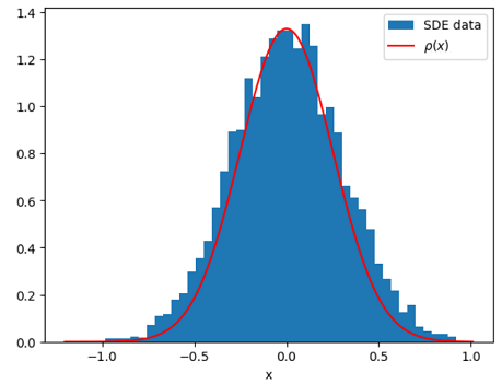
I also calculated the histogram of the probability density of the random variable $x(t)$ evaluated at $t = 10$ using the $5000$ simulated sample paths, and plotted it together with the stationary pdf, $\rho(x)$ , derived above from the Fokker-Planck equation. The plot below shows good agreement between the two:

Ornstein-Uhlenbeck process: derivation and simulation of its pdf and moments

Published by Dr Christian P. H. Salas

Leave a comment Cancel reply