From simple random walk to Wiener process and diffusion equation

For the purposes of a lecture, I wanted a very straightforward mathematical setup leading quickly from a simple random walk to the Wiener process and also to the associated diffusion equation for the Gaussian probability density function (pdf) of the Wiener process. I wanted something simpler than the approach I recorded in a previous post for passing from a random walk to Brownian motion with drift. I found that the straightforward approach below worked well in my lecture and wanted to record it here.

The key thing I wanted to convey with the random walk model is how the jumps at each step have to be of a size exactly equal to the square root of the step length in order for the limiting process to yield a variance for the stochastic process that is finite at the limit but not zero. To this end, suppose we have an interval of time $[0, T]$ and we divide it into $N$ subintervals of length $\Delta t$ , so that

$\Delta t = \frac{T}{N} \quad \quad \quad \quad (1)$

The situation is illustrated in the following sketch:

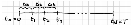
For each time step $t_n = n \Delta t$ , define the simple random walk

$x_{n+1} = x_n + \Delta W_{n+1} \quad \quad \quad \quad (2)$

where for $n = 0, 1, 2, \ldots,$ we have

$\Delta W_{n+1} = \begin{cases} \quad \Delta h & \text{with probability } \frac{1}{2} \\ \quad & \quad \\ -\Delta h & \text{with probability } \frac{1}{2}\end{cases}$

The mean and variance of $\Delta W_{n+1}$ are easily calculated as

$E[\Delta W_{n+1}] = \frac{1}{2} (\Delta h) + \frac{1}{2} (-\Delta h) = 0 \quad \quad \quad \quad (3)$

and

$V[\Delta W_{n+1}] = E[\Delta W_{n+1}^2] - E^2[\Delta W_{n+1}]$

$= \frac{1}{2} (\Delta h)^2 + \frac{1}{2} (-\Delta h)^2 - 0$

$= (\Delta h)^2 \qquad \qquad \qquad \qquad \qquad \qquad \qquad (4)$

The recurrence relation in (2) represents a progression through a simple random walk tree starting at $x_0$ , as illustrated in the following picture:

Running the recurrence relation with back substitution we obtain

$\Delta x_T = \sum_{k=1}^{N} \Delta W_k \quad \quad \quad \quad (5)$

where $\Delta x_T \equiv x_N - x_0$ . The mean and variance of $\Delta x_T$ are again easily calculated as

$E[\Delta x_T] = \sum_{k=1}^{N} E[\Delta W_k] = 0 \quad \quad \quad \quad (6)$

and

$V[\Delta x_T] = \sum_{k=1}^{N} V[\Delta W_k] = N(\Delta h)^2 = \frac{T}{\Delta t} (\Delta h)^2 \quad \quad \quad \quad (7)$

This final expression for the variance is the one I wanted to get to as quickly as possible. It shows that for the variance to remain finite but not zero as we pass to the limit $\Delta t \rightarrow 0$ , it must be the case that $\Delta h = \sqrt{\Delta t}$ . From (7) we then obtain

$V[x_T] = T \quad \quad \quad \quad (8)$

which is the characteristic variance of a Wiener process increment over a time interval $[0, T]$ . Any other choice of $\Delta h$ would lead to the variance of the random walk either exploding (if $\Delta h \neq 0$ ) or flatlining (if $\Delta h = 0$ ), rather than settling into a Wiener process as $\Delta t \rightarrow 0$ .

Next, I wanted to show how the Gaussian pdf of the Wiener process follows immediately from the above random walk structure (without any need to appeal to the central limit theorem for the sum in (5)). Over an interval of time $T - \Delta t$ to $T$ , the simple random walk underlying the Wiener process can reach a point $x$ by increasing from the point $x - \Delta h$ or by decreasing from the point $x + \Delta h$ , as illustrated in the following picture:

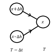
Each of these has a probability of $\frac{1}{2}$ , so the probability density function $p(x, T)$ we are looking for must satisfy

$p(x, T) = \frac{1}{2} p(x - \Delta h, T - \Delta t) + \frac{1}{2} p(x + \Delta h, T - \Delta t) \quad \quad \quad \quad (9)$

We now Taylor-expand each of the terms on the right-hand side about $(x, T)$ to obtain

$p(x - \Delta h, T - \Delta t)$

$= p(x, T) - \frac{\partial p}{\partial x} \Delta h - \frac{\partial p}{\partial t} \Delta t + \frac{1}{2!} \frac{\partial^2 p}{\partial x^2} (\Delta h)^ 2 + \cdots \quad \quad \quad \quad (10)$

and similarly

$p(x + \Delta h, T - \Delta t)$

$= p(x, T) + \frac{\partial p}{\partial x} \Delta h - \frac{\partial p}{\partial t} \Delta t + \frac{1}{2!} \frac{\partial^2 p}{\partial x^2} (\Delta h)^ 2 + \cdots \quad \quad \quad \quad (11)$

Note that we will be setting $\Delta h$ equal to $\sqrt{\Delta t}$ and letting $\Delta t \rightarrow 0$ , so we do not need to include any of the higher-order $\Delta h$ or $\Delta t$ terms in these Taylor expansions. Substituting (10) and (11) into (9) and setting $\Delta h = \sqrt{\Delta t}$ gives

$p(x, T) = p(x, T) - \frac{\partial p}{\partial t} \Delta t + \frac{1}{2!} \frac{\partial^2 p}{\partial x^2} \Delta t$

which simplifies to

$\frac{1}{2} \frac{\partial^2 p}{\partial x^2} = \frac{\partial p}{\partial t} \quad \quad \quad \quad (12)$

This is the diffusion equation for the standard Wiener process which has as its solution the Gaussian probability density function

$p(x, t) = \frac{1}{\sqrt{2 \pi t}} \exp \big(-\frac{x^2}{2t}\big) \quad \quad \quad \quad (13)$

This can easily be confirmed by direct substitution (cf. my previous post where I play with this).

From simple random walk to Wiener process and diffusion equation

Published by Dr Christian P. H. Salas

Leave a comment Cancel reply