Quantum mechanical models in three dimensions and involving many particles, etc., use a formalism which is largely based on some key mathematical modelling ideas pertaining to single particle systems. These mathematical modelling ideas are principally designed to tell us what sets of values we are `allowed’ to observe when we measure some aspect of a quantum system, and with what probabilities we can expect to observe particular values from these sets. For quick reference, I wanted to have a relatively brief and coherent overview of these key mathematical ideas and have written the present note for this purpose. Dirac notation is used throughout.
Quantum particle in a ring
To start with, suppose all we know is that a quantum particle in a closed ring of length  has a given linear momentum
  when an observation of its position is made. The result of the observation is that the particle will be found at some point
  lying in a small interval of length
  on the closed ring. We assume that the radius of the ring is sufficiently large to make angular momentum considerations negligible. De Broglie tells us that the linear momentum of the quantum particle must be associated with a wavelength
  of some wave function
  according to the rule

where  is Planck’s constant. (There is also a fundamental equation
  linking the energy of a quantum particle to the frequency of a wave function. This will be introduced later in connection with modelling time evolution in quantum mechanics). Somewhat surprisingly at first sight, this is all the information we need to deduce a precise functional form for the wave function as well as the allowed spectrum of momenta for the particle. (Note that
  gives the probability that a particle with momentum will be found at a position lying in a small interval of length on the closed ring. This probability distribution can be observed through experiment, while itself is unobservable directly. We refer to as a quantum mechanical probability amplitude in this connection).
First, we imagine what the position wave function must look like as a Fourier series. Since only a single wavelength is involved in this particular setup, must be a pure wave, i.e., the exponential form of its Fourier series must consist of a single term, so we must have

for some  that still remains to be calculated, where
  is the wave number

Combining (1) and (3), we can write de Broglie’s linear momentum formula as

where  is the reduced Planck’s constant. We can then rewrite the above wave function to explicitly incorporate momentum as

An assumption called the certainty condition in quantum mechanics, or sometimes the square integrability condition or normalizability condition, is that the quantum particle must be found upon measurement to be located somewhere on the ring, so we must have

(This requires quantum mechanics to take place in a Hilbert space of square-integrable functions, as discussed further below). Substituting our wave function so far into this then gives  , so we can write the full position wave function as

Second, to deduce the permitted spectrum of momenta, we use the fact that the position wave function for a quantum particle in a ring must be periodic with period , so we must have

Therefore

which implies

for  , and therefore the permitted spectrum of momenta for this setup is given by

It is impossible for this quantum particle to have a momentum that does not belong to this particular discrete spectrum.
In our one-dimensional quantum particle in a ring system, a measurement result that is nondegenerate uniquely defines a state of the system, denoted by a ket  in Dirac notation, e.g.,
  for a momentum measurement or
  for a position measurement. Formally, as outlined below, these kets are vectors in a Hilbert space. In contrast, a degenerate measurement is a measurement that cannot uniquely define a state of the system, i.e., it is consistent with more than a single state and is thus regarded as a superposition of states. As an example, the energy
  of our particle in a ring system is degenerate because it is a quadratic function of momentum,
  , and there is nothing in the model to prevent the momentum being negative. Thus, the same value of can correspond to a momentum state or a momentum state
  , so the label cannot by itself be used to uniquely define a state
  here.
here.
An event is a measurement finding for a system when it is in a known, i.e., pre-prepared, state. For example, we can measure the position for our system when we know the quantum particle in the ring has been prepared to have momentum state . In quantum mechanics, all such events have probability amplitudes with the property that their absolute value squared gives a probability density for the event, as mentioned above. In this case, as mentioned earlier, the probability amplitude for the position measurement is in Dirac notation, with  . Note that there is an implicit assumption that the measurement of position occurs instantaneously after the quantum system has been prepared in its initial momentum state, i.e., there should not have been enough time for the system to evolve away from its pre-prepared momentum state before position is measured. This implicit assumption applies to all quantum events. Also note that the famous Dirac delta function in the continuous case (and the Kronecker delta function in the discrete case) arise by considering self-space events, i.e., performing the same measurement twice in rapid succession. For example, suppose the quantum particle is known to be in position state
  and then a second measurement of position is quickly made. The measurement space in this case is continuous and the self-space probability amplitude
  is given by the Dirac delta function

which is such that  for
for  , while
  for
for  in such a way that
  , and which famously also has as its defining property the integral equation

In the case of repeated measurements of momentum, which has a discrete measurement space for the quantum particle in a ring model, the corresponding self-space probability amplitude would be given by the Kronecker delta

which is such that  if
if  , and
, and  if
if  . The Dirac delta function can be thought of as the continuous measurement space analogue of the Kronecker delta for discrete spaces.
The abstract measurement space consisting of the spectrum of all possible results you can get from a measurement is a Hilbert space, i.e., a complex inner product space which is also a complete metric space with regard to the distance function induced by the inner product. The state of a physical system is treated as a vector in such a Hilbert space. There is a Hilbert space containing all the possible position and momentum states above, for example, and the probability amplitudes are formally the inner products of the two state vectors and in this Hilbert space. A necessary and sufficient condition for these inner products to exist is that the functions involved are square-integrable. The completeness of these measurement spaces means that each can act as a basis, i.e., a ‘language’, in terms of which other states can be represented. Thus, we can regard the probability amplitude as the projection of state on -space, or the momentum state expressed in the language of , or simply the state expressed as a function of . Similarly,  can be interpreted as the position state expressed in the language of . A key axiom of quantum mechanics is that and are related via complex conjugation:

So, for example, given as defined in (7) above, we can immediately deduce that

(But remember that these probability amplitudes are never directly observable. Only the associated probability distributions are observable experimentally).
We can use this idea of measurement spaces acting as language spaces (or, more formally, basis sets) to express one state as a superposition of other states. For example, a hypothetical state  can be experimentally resolved into momentum state components, expressed mathematically as the superposition

This is a discrete sum because recall that, for the quantum particle in a ring model, the measurement space for momentum is discrete. On the right-hand side, each is a pure momentum state, and the bra-ket  is the weight attached to this pure momentum state in the superposition. The same state can equally well be perceived as a superposition of position states:

The summation here is to be implemented as an integral since the measurement space for position is continuous for the quantum particle in a ring model. Thus, we can write (14) in integral form as

Notice how the delta function definition of the self-space amplitude,  , now arises in this integral when computing the coefficients of the expansion of
  in terms of the continuous position basis:

Thus, the position space wave functions  , evaluated at particular values of , are just the coefficients of a state (belonging to Hilbert space) in a superposition using a continuous position basis.
It is useful to bear in mind that these superposition equations are analogous to how a periodic function  can be expanded in a Fourier series. We are using the same kinds of mathematical structures and arguments in defining the superpositions above.
Both of the superposition equations above are special cases of a general rule called the completeness theorem or superposition theorem, which can be expressed mathematically in Dirac notation as

The ket  on the left-hand side of this equation is a pure
  -state. The bra
  can be regarded here as an operator that, when it is applied to any state , gives the weight attached to that pure -state in the superposition for :

In this last equation, it is as if we are multiplying on the right-hand side by 1 to get again on the left-hand side, so we represent this situation as in equation (15) above.
Measuring an observable for our quantum system, assuming the system has been prepared so that it is in a known state when the measurement takes place, is modelled mathematically as applying a suitable operator to the prepared state ket. If an operator  operates on a state ket , another new state ket is produced denoted by
  . For each such operator , there must be a rule or instruction which tells us what is produced when the ket undergoes the operation. This rule must itself be given in some language, e.g., the representation of in -space is denoted
  , and in -space is denoted
  . An important example is the operator
  whose rule in -space is take the derivative with respect to x. Therefore, in Dirac notation:

This equation can be applied to any ket, so for example

In the same way that a state has an existence which is independent of the language used to represent it, so too may operators be expressed in different languages. For example, we can convert an instruction in -language to an instruction in -language by using a ket-bra sum  . We get

No specific state is involved here, so we can write the general language-translation-rule as

To give an example of implementing this in practice, recall that for our quantum particle in a ring system we have

Therefore, the conversion represented by (19) can be written in conventional notation as

Integrating the right-hand side by parts, we find it equals


Therefore,

Since is arbitrary, the general rule is

The operators that represent measurement of observables in quantum mechanics are linear and hermitian. (A hermitian matrix is the complex analogue of a symmetric matrix. It is equal to its own conjugate transpose. Another type of matrix which arises frequently in quantum mechanics is a unitary matrix. This is the complex analogue of an orthogonal matrix, the latter having the property that the transpose matrix is the inverse. In the case of a unitary matrix, the complex conjugate transpose is the inverse. Hermitian operators are usually related to the measurement of observables in quantum mechanics, whereas unitary operators are related to carrying out processes such as translations of quantum states in space and time. We need to extend the symmetric and orthogonal properties of ordinary matrices to include complex conjugation in the definition of hermitian and unitary matrices to cater for the fact that quantum mechanics involves complex numbers, e.g., in the unitary matrix case, simply transposing a complex matrix and multiplying by the original matrix would in general produce another complex matrix rather than an identity matrix, without the complex conjugation step). As per Sturm-Liouville theory, hermitian operators have the property that their eigenvalues are real and form complete measurement spaces, i.e., they represent the entire spectrum of values that can be observed when a measurement is made. It is important to understand, however, that these eigenvalues are only revealed when the operator is applied to its particular home measurement space, formally called its eigenspace. Each operator is defined in terms of a particular instruction (telling us what the operator does) and in terms of the set of eigenvalues it gives rise to when it is applied to its particular eigenspace. The effect of applying an operator to a ket in its eigenspace will be to produce the same ket multiplied by an eigenvalue of the operator. The kets for which this happens are the eigenkets of the operator. For example, based on the result in (22) above, define a new operator  as
as

Then on the basis of (22), we immediately deduce that

This is the bra form of the eigenvalue equation for , meaning that in -language, which is the language of the eigenspace of , the effect of is to multiply any state it operates on by a number . We can equivalently state the eigenvalue equation in ket form:

This is saying that the effect of on its eigenket is to produce a number times the same eigenket, no matter what language the instruction for is expressed in. The two forms (24) and (25) are equivalent, and both mean that the operator produces the spectrum of momenta for the quantum particle in a ring model, and the eigenkets of are . We say that the -space kets are eigenstates of with eigenvalues . Notice that when the operator is expressed in -language instead of -language, we do not get a proper eigenvalue equation (see (18) above). Therefore, -space is not the eigenspace of . However, when the operator is expressed in -language, we do get a proper eigenvalue equation (equation (22) above), so -space is the eigenspace for .
Similarly, since position is a measurable quantity for the quantum particle in a ring, there is a position operator  which generates a position measurement space, just as generates momentum measurement space. The eigenvalue equation for is simply

Note that each of and can be expressed in the language of the other’s space. Expressing in -language, we find

(Proof:  ). Similarly, expressing in -language we get

(Proof:  ). In each case, we are not using the correct eigenspace for the operator, so the equations we get are not in the form of proper eigenvalue equations. However, we can check that (27) and (28) are correct by seeing if they do produce proper eigenvalue equations when applied to the correct kets. When applied to the ket , equation (27) must produce the proper eigenvalue equation

Therefore we need to confirm that

but this result is immediate when we substitute (12) into each side of (30). Similarly, when applied to the ket , equation (28) must produce the proper eigenvalue equation

Therefore we need to confirm that

but this is again immediate when we substitute (7) into each side of (32).
Another interesting thing to observe here is that we can reverse this argument and derive the form of the probability amplitude as a function of from (32), interpreted as a differential equation. We can regard (32) as the the eigenvalue equation in (25) above, but expressed in the language of (i.e., the differential equation in (32) is obtained by introducing the bra  in (25) above, yielding
  ). The solution to (32) is precisely the form of given in (7) above, with the constant coming from the normalization condition
  as before.
In addition to position and momentum operators and , energy is also an observable, so it must have an operator that generates the spectrum of measurable energies. This is the Hamiltonian operator, which for a quantum particle in a ring model has the form

(There is no potential energy in our simple model system, so no function of in the Hamiltonian). Note that the form of the operator  is the same as the form of the classical kinetic energy function
  . In the quantum case, the eigenvalues of are precisely . Remarkably, a simple rule that works for finding quantum mechanical operators corresponding to classical observables is to put hats on the observables in algebraic relations between classical observables. This is how we can get from . As another example, we could in principle obtain a quantum velocity operator as
  .
.
Having the form of the Hamiltonian operator , we can now find its eigenvalues from the eigenvalue problem that generates them:

This is actually the general form of the famous time-independent Schrödinger equation. Casting this equation into -space, we can solve for the probability amplitudes  :
:

This is a simple second-order linear differential equation with general solution

From the fact that this wave function must be single-valued for our quantum particle in a ring, we deduce

for . Remember, however, that there is degeneracy in for the quantum particle in a ring model: there is nothing to prevent there being two possible -states (one positive, one negative) for each value of .
Quantum particle on an infinite line
Suppose we modify the previous model by allowing the radius of the ring,  , to become infinitely large, so that the `track’ now effectively extends infinitely to the right and infinitely to the left of the starting point at zero. The quantum particle is then free to move anywhere on the real line, i.e., the position measurement space has become
  . For such a quantum particle, momentum is no longer quantized (intuitively, this is because the probability amplitude periodicity constraint
  is no longer relevant), so the momentum measurement space is now
  . In this context, with both position and momentum being continuous measurement spaces, Fourier transforms arise naturally because they enable any function of over the domain , such as
  , to be expanded as an integral in over the same domain:

where  is given by

We can use this Fourier transform relationship to obtain physically-realistic mathematical models of a quantum particle on an infinite line. As is well known, in order to obtain a well-behaved wave function representation of a free particle on an infinite line, i.e., a wave function that is square-integrable, it is necessary to construct a superposition of pure waves incorporating a continuous range of wave numbers . This wave packet approach then naturally gives rise to discussions relating to Heisenberg’s uncertainty principle. Before considering this, however, it is interesting to note that we can also derive a pseudo-normalized pure wave form for the wave function in the case of a quantum particle on an infinite line, somewhat analogous to the pure wave form in the previous section. To do this, we will first obtain a representation of the Dirac delta function using the above Fourier transform by letting  . Putting this into (38) gives

Then, putting this result into (37) gives us the following useful representation:

We will also observe that for any  , we have

(To see this, note first that  because
  . Therefore, only the absolute value of
  in
in  is relevant. We need to show that
  . In the integral on the left-hand side, make the change of variable
  . Then
  and
and  , and noting that
  , i.e., both are functions of , we can write as required).
We now use this machinery to derive an explicit pure wave functional form for . First, consider the self-space bra-ket

where the final equality follows from (41). Using (40), reversing the roles of and there, we can write


![= \int_{-\infty}^{\infty} dx \big[\frac{1}{\sqrt{h}}\exp(-i k x)\big]\big[\frac{1}{\sqrt{h}} \exp(i K x) \big]\qquad \qquad \qquad \qquad \qquad (43)](https://s0.wp.com/latex.php?latex=%3D+%5Cint_%7B-%5Cinfty%7D%5E%7B%5Cinfty%7D+dx+%5Cbig%5B%5Cfrac%7B1%7D%7B%5Csqrt%7Bh%7D%7D%5Cexp%28-i+k+x%29%5Cbig%5D%5Cbig%5B%5Cfrac%7B1%7D%7B%5Csqrt%7Bh%7D%7D+%5Cexp%28i+K+x%29+%5Cbig%5D%5Cqquad+%5Cqquad+%5Cqquad+%5Cqquad+%5Cqquad+%2843%29&bg=ffffff&fg=111111&s=0&c=20201002)
But we also have in Dirac notation

Comparing (43) and (44) we can immediately see that

The only difference between here and in (7) above for the quantum particle in a ring case is that the normalization constant here is  instead of
  . It is easily checked that (45) is in fact not square-integrable for the case of the quantum particle on an infinite line, i.e., is not an element of a Hilbert space in the conventional way here, since
  . Instead, a kind of pseudo-normalization convention is being used in specifying the normalization constant in (45), called normalization to a Dirac delta function. From (43) (remembering that
  ) we see that the normalization constant in (45) is giving us normalization to a Dirac delta function in the form

However, the non-square-integrable individual pure waves in (45) do not represent physically realizable states. To construct a square-integrable wave packet representation of a quantum particle on a line, we go back to the Fourier transform equation (37) above and regard it as a sum of pure waves over a continuous range of wave numbers , with the amplitudes of these pure waves being modulated by the function . A standard example is a Gaussian wave packet which we can obtain here by specifying

where  is some fixed wave number. Note that
  is the probability density function of a
  variable, i.e., up to a normalizing constant we get a Gaussian probability distribution for the wave number centered on with standard deviation
  . Inserting this expression for in (37) gives

The integral here can be solved using straightforward changes of variables to give the result

This is a localized wave function and is square-integrable since  is the probability density function of a
  variable, i.e., we get a Gaussian probability distribution for the position centered at zero and with standard deviation
  . (As a check, note that substituting this expression for into (38) must give us the expression we used for . Using the the result

and the fact that  , we can substitute the expression for into (38) to get


as required). Denoting the standard deviation of by  and the standard deviation of by
  , we have

But using  , we can write this as

It can be shown that for anything other than a Gaussian wave packet we would find

and thus we obtain the famous Heisenberg uncertainty principle for position and momentum:

This wave packet model is a static one, i.e., the wave function is time-independent. We can obtain a time-dependent wave function  by multiplying the integrand in (37) by a quantum mechanical time evolution operator (the time evolution operator will be discussed below). Then, using the same as in the static case and manipulating the integral in a similar manner as before, we find that is again a localized Gaussian wave packet but now with the property that the standard deviation of the associated Gaussian probability distribution increases with time (i.e., the bell-shaped Gaussian probability distribution spreads out over time).
Quantum harmonic oscillator
To extend the model further, we now consider a quantum harmonic oscillator in which the position still has domain . In this model, the momentum is again no longer quantized but energy remains quantized and is no longer a degenerate measurement. The approach is essentially to take the ideal classical harmonic oscillator’s Hamiltonian, convert it to a quantum mechanical Hamiltonian operator by `putting hats’ on the classical observables, and then use the operator to solve an eigenvalue problem.
Recall that, in the ideal classical harmonic oscillator model, a particle of mass  attached to a spring with spring constant
  is always pulled towards an equilibrium position by a Hooke’s law force
  . Newton’s second law
  then gives us a second-order differential equation

with general solution

The angular frequency (or, equivalently, angular velocity – radians per second) is thus

and is usually referred to as the natural oscillation frequency of the harmonic oscillator.
The particle’s kinetic energy is where is the classical linear momentum, and, unlike the previous models, we now have a potential energy  . (Recall that potential energy is the negative of work,
  . For the classical harmonic oscillator, we have
  , so the potential energy is the negative of this). The classical Hamiltonian is then

Using (49), we can write the corresponding quantum mechanical Hamiltonian operator as

As before, the position spectrum is generated by and the momentum spectrum is generated by . The energy spectrum is generated by via the time-independent Schrödinger equation, which is the following eigenvalue problem for :

In Dirac notation, this general eigenvalue problem statement does not yet specify a `language’ in which to express the solutions. We can cast the eigenvalue problem into -space by introducing the bra  and expressing the operator in -language. We get the time-independent Schrödinger equation as the second-order differential equation

This is a well-known differential equation in disguise. The general form is

It is easily seen that (53) becomes (54) if we take

and

The solutions of (54) are stated in terms of the Hermite polynomials,  ,
,  ,
,  ,
,  . The solutions in terms of are

where only solutions with nonnegative integer values of  make square-integrable, so only these solutions are allowable. We see that is indeed quantized, i.e., indexed by nonnegative integers , so if we wanted to we could write as
  to emphasise the relevant energy index. The
  sequence of energies means that can never be zero for the quantum harmonic oscillator, and it can only go up in discrete steps of
  from its minimum value of
  . Also note that, as stated earlier, the ladder of values is not degenerate for the quantum harmonic oscillator (unlike the particle in a ring model) because only nonnegative integers yield valid solutions for this particular eigenvalue problem.
The quantum harmonic oscillator is also used to introduce additional quantum concepts such as quantum tunnelling (the probability amplitudes are nonzero outside the quadratic potential well for this model, so there is a nonzero probability that the quantum particle can be found outside the potential well. This would be impossible for the classical harmonic oscillator). Another thing to observe here is that it is also possible to cast the eigenvalue problem in -language instead of -language (resulting in expressions for the probability amplitudes  which are isomorphic to those for ), and in energy-level language, which introduces the ideas of creation and annihilation operators (also known as raising and lowering operators, respectively, or as ladder operators), as well as commutators. These are nonphysical operators, i.e., they do not correspond to observables, but rather are regarded as useful computational aids.
The annihilation operator  for the quantum harmonic oscillator can be defined in terms of and as

and the creation operator is its hermitian conjugate

These can be derived from the Hamiltonian operator by pseudo-factorising it. See my previous note about this. From these two equations, we can show that their commutator is unity, i.e.,
![[\hat{a}, \hat{a}^{\dag}] = \hat{a} \hat{a}^\dag - \hat{a}^{\dag} \hat{a} = 1 \qquad \qquad \qquad \qquad \qquad (60)](https://s0.wp.com/latex.php?latex=%5B%5Chat%7Ba%7D%2C+%5Chat%7Ba%7D%5E%7B%5Cdag%7D%5D+%3D+%5Chat%7Ba%7D+%5Chat%7Ba%7D%5E%5Cdag+-+%5Chat%7Ba%7D%5E%7B%5Cdag%7D+%5Chat%7Ba%7D+%3D+1+%5Cqquad+%5Cqquad+%5Cqquad+%5Cqquad+%5Cqquad+%2860%29&bg=ffffff&fg=111111&s=0&c=20201002)
and the Hamiltonian operator itself can now be re-expressed in terms of these ladder operators as

We also find
![[\hat{a}, \hat{H}] = \hbar \omega \hat{a} \qquad \qquad \qquad \qquad \qquad (62)](https://s0.wp.com/latex.php?latex=%5B%5Chat%7Ba%7D%2C+%5Chat%7BH%7D%5D+%3D+%5Chbar+%5Comega+%5Chat%7Ba%7D+%5Cqquad+%5Cqquad+%5Cqquad+%5Cqquad+%5Cqquad+%2862%29&bg=ffffff&fg=111111&s=0&c=20201002)
![[\hat{a}^{\dag}, \hat{H}] = -\hbar \omega \hat{a}^{\dag} \qquad \qquad \qquad \qquad \qquad (63)](https://s0.wp.com/latex.php?latex=%5B%5Chat%7Ba%7D%5E%7B%5Cdag%7D%2C+%5Chat%7BH%7D%5D+%3D+-%5Chbar+%5Comega+%5Chat%7Ba%7D%5E%7B%5Cdag%7D+%5Cqquad+%5Cqquad+%5Cqquad+%5Cqquad+%5Cqquad+%2863%29&bg=ffffff&fg=111111&s=0&c=20201002)
These results allow us to avoid all mention of and when investigating the energy measurement space generated by the operator in the eigenvalue problem given as equation (52) above. We have
![[\hat{a}, \hat{H}] | E \rangle = \hbar \omega \hat{a} | E \rangle](https://s0.wp.com/latex.php?latex=%5B%5Chat%7Ba%7D%2C+%5Chat%7BH%7D%5D+%7C+E+%5Crangle+%3D+%5Chbar+%5Comega+%5Chat%7Ba%7D+%7C+E+%5Crangle&bg=ffffff&fg=111111&s=0&c=20201002)
and thus

so

Similarly, from
![[\hat{a}^{\dag}, \hat{H}] | E \rangle = -\hbar \omega \hat{a}^{\dag} | E \rangle](https://s0.wp.com/latex.php?latex=%5B%5Chat%7Ba%7D%5E%7B%5Cdag%7D%2C+%5Chat%7BH%7D%5D+%7C+E+%5Crangle+%3D+-%5Chbar+%5Comega+%5Chat%7Ba%7D%5E%7B%5Cdag%7D+%7C+E+%5Crangle&bg=ffffff&fg=111111&s=0&c=20201002)
we have

and so

Therefore, applied to produces a new eigenket  which is lowered in energy by . Similarly,
  produces an eigenket raised in energy by . As mentioned earlier, we can use the integer index to label the energy states instead of , i.e., we can write
  instead of . To make the ladder effect of the creation and annihilation operators even more obvious, we can then write


and try to work out the eigenvalues  and
and  . The value of can be deduced by noting that applying in the form of (61) above to and using (55) we get

which reduces to

But  , so we must have
  . Therefore (66) can be written explicitly as

We now use this result to deduce the value of by writing it as

Adding a bra  gives us a self-space bracket on the right-hand side:

But  , so for (68) to be nonzero we must have
  , so
, so  , and notice that this must also be true for
  to be nonzero, so
  and must both represent the same function. With these insights, we can re-express (68) as

Taking the hermitian conjugate of both sides of (69) gives

from which we deduce that the explicit form of (67) must be

i.e.,  . Thus, we have


Quantum particle on a spherical shell
We now extend the model further by introducing two-dimensional quantum states for a quantum particle on a spherical shell. The general approach to modelling is similar to the approach for the harmonic oscillator in a number of ways. In particular, we begin by setting up a classical model of a particle on a sphere, and then quantize it by considering the relevant quantum mechanical operators in a quantum version of the model.
In a classical model of a particle on a spherical shell, the particle is constrained to positions at a fixed distance  from the origin, but can otherwise move anywhere on a spherical surface. In the previous quantum particle in a ring model,
  was assumed to be sufficiently large to enable angular momentum considerations to be ignored, and the focus was then on linear momentum . In the present particle on a spherical shell model, we no longer assume is large and in fact the particle now only has angular momentum. As discussed in a previous post involving angular momentum calculations, the classical particle has a vector angular momentum about the origin given by

which has components


There is no potential energy in this model, only kinetic energy, but the constraint that the particle must remain on the spherical shell means that  and
and  are always orthogonal, so

This linear constraint means that only two of the three linear momentum components are linearly independent, so the linear momentum space for this model is two-dimensional. In view of (71) and (75), the magnitudes of the linear and angular momentum are related by

so

Therefore, the Hamiltonian for the classical particle in a shell model is

Using spherical coordinates, the classical particle can wander anywhere on the sphere, with any angular momentum in any direction, its position characterised by the polar angle  and the azimuthal angle
  . In the case of a quantum particle on a spherical shell, a position measurement defines a two-dimensional basis space and a position state would be denoted by the ket
  . There would be two quantum operators
  and
and  whose eigenvalues are the spectra of possible and values respectively, and a single eigenstate is now regarded as a simultaneous solution of the two eigenvalue problems for these operators:


This is possible if and only if and commute, i.e., ![[\hat{\theta}, \hat{\varphi}] = 0](https://s0.wp.com/latex.php?latex=%5B%5Chat%7B%5Ctheta%7D%2C+%5Chat%7B%5Cvarphi%7D%5D+%3D+0&bg=ffffff&fg=111111&s=0&c=20201002) . Operators which commute are called compatible operators and they must have simultaneous eigenstates. Conversely, two operators which have simultaneous eigenstates must commute. (An indication of why this is true is as follows. Suppose we are given the eigenvalue equation (78), so that is an eigenstate of with eigenvalue . Then, given , we must have
. Operators which commute are called compatible operators and they must have simultaneous eigenstates. Conversely, two operators which have simultaneous eigenstates must commute. (An indication of why this is true is as follows. Suppose we are given the eigenvalue equation (78), so that is an eigenstate of with eigenvalue . Then, given , we must have

Therefore, both  and are eigenstates of with the same eigenvalue , so they must represent the same eigenstate up to some proportionality constant. The fact that and represent the same eigenstate up to a proportionality constant is exactly what (79) says). The fact that this condition holds means that the measurement of an eigenvalue of does not destroy knowledge of an eigenvalue of , and vice versa. This is not possible with all pairs of measurements. For example, the operators and are incompatible and thus do not have simultaneous eigenstates, so no two-dimensional state such as
  exists. Knowledge of would be destroyed by a measurement of , and vice versa. This is indicated by the fact that and do not commute, since
 ![[\hat{x}, \hat{p}] = i \hbar \neq 0](https://s0.wp.com/latex.php?latex=%5B%5Chat%7Bx%7D%2C+%5Chat%7Bp%7D%5D+%3D+i+%5Chbar+%5Cneq+0&bg=ffffff&fg=111111&s=0&c=20201002) . Simultaneous eigenstates can only exist for operators which commute.
. Simultaneous eigenstates can only exist for operators which commute.
Note that this idea of compatible vs incompatible operators is intimately related to Heisenberg’s uncertainty principle. Given two operators  and
and  , with standard deviations
  and
and  respectively, the generalised form of Heisenberg’s uncertainty principle says
![\Delta a \Delta b \ge \frac{1}{2} |\langle [\hat{A}, \hat{B}] \rangle|](https://s0.wp.com/latex.php?latex=%5CDelta+a+%5CDelta+b+%5Cge+%5Cfrac%7B1%7D%7B2%7D+%7C%5Clangle+%5B%5Chat%7BA%7D%2C+%5Chat%7BB%7D%5D+%5Crangle%7C&bg=ffffff&fg=111111&s=0&c=20201002)
where ![|\langle [\hat{A}, \hat{B}] \rangle|](https://s0.wp.com/latex.php?latex=%7C%5Clangle+%5B%5Chat%7BA%7D%2C+%5Chat%7BB%7D%5D+%5Crangle%7C&bg=ffffff&fg=111111&s=0&c=20201002) denotes the absolute value of the expectation of the commutator of and . (The concept of the expectation of an operator is discussed in a later section below). Thus, there is no uncertainty principle for compatible operators, and measurement of one will not affect measurement of the other. However, there is always an uncertainty principle for incompatible operators, i.e., those with non-zero commutators, and it is impossible to measure one without destroying a previous measurement of the other.
denotes the absolute value of the expectation of the commutator of and . (The concept of the expectation of an operator is discussed in a later section below). Thus, there is no uncertainty principle for compatible operators, and measurement of one will not affect measurement of the other. However, there is always an uncertainty principle for incompatible operators, i.e., those with non-zero commutators, and it is impossible to measure one without destroying a previous measurement of the other.
Recall that in the case of the harmonic oscillator we could solve the eigenvalue problem in -language, -language, or energy-level-language, and the energy-level-language approach gave rise to creation and annihilation operator approaches. Similar considerations apply to the quantum particle on a spherical shell model. We can solve the eigenvalue problem in the language of angular momentum components rather than in the language of spatial or linear momentum states, and this gives rise to ladder operators analogous to the creation and annihilation operators for the quantum harmonic oscillator. Since angular momentum components can be measured, there must be angular momentum state labels and angular momentum operators. The angular momentum operators are simply the classical angular momenta turned into operators by `putting hats on them’. Thus, we get the operators


The eigenvalues of  make up the measurement spectrum of the square of the total angular momentum.
We know that spatial states and linear momentum states are two-dimensional, so we must also find that the measurement space created by the angular momentum operators is two-dimensional since dimensionality is conserved, no matter what language is used to describe the system. Indeed, we find that no two of the three angular momentum operators commute with each other:
![[\hat{L}_x, \hat{L}_y] = i\hbar \hat{L}_z \qquad \qquad \qquad \qquad \qquad (84)](https://s0.wp.com/latex.php?latex=%5B%5Chat%7BL%7D_x%2C+%5Chat%7BL%7D_y%5D+%3D+i%5Chbar+%5Chat%7BL%7D_z+%5Cqquad+%5Cqquad+%5Cqquad+%5Cqquad+%5Cqquad+%2884%29&bg=ffffff&fg=111111&s=0&c=20201002)
![[\hat{L}_y, \hat{L}_z] = i\hbar \hat{L}_x \qquad \qquad \qquad \qquad \qquad (85)](https://s0.wp.com/latex.php?latex=%5B%5Chat%7BL%7D_y%2C+%5Chat%7BL%7D_z%5D+%3D+i%5Chbar+%5Chat%7BL%7D_x+%5Cqquad+%5Cqquad+%5Cqquad+%5Cqquad+%5Cqquad+%2885%29&bg=ffffff&fg=111111&s=0&c=20201002)
![[\hat{L}_z, \hat{L}_x] = i\hbar \hat{L}_y \qquad \qquad \qquad \qquad \qquad (86)](https://s0.wp.com/latex.php?latex=%5B%5Chat%7BL%7D_z%2C+%5Chat%7BL%7D_x%5D+%3D+i%5Chbar+%5Chat%7BL%7D_y+%5Cqquad+%5Cqquad+%5Cqquad+%5Cqquad+%5Cqquad+%2886%29&bg=ffffff&fg=111111&s=0&c=20201002)
Therefore, it is impossible to define eigenstates based on these components. However, all three components do commute with :
![[\hat{L}_x, \hat{L}^2] = [\hat{L}_y, \hat{L}^2] = [\hat{L}_z, \hat{L}^2] = 0 \qquad \qquad \qquad \qquad \qquad (87)](https://s0.wp.com/latex.php?latex=%5B%5Chat%7BL%7D_x%2C+%5Chat%7BL%7D%5E2%5D+%3D+%5B%5Chat%7BL%7D_y%2C+%5Chat%7BL%7D%5E2%5D+%3D+%5B%5Chat%7BL%7D_z%2C+%5Chat%7BL%7D%5E2%5D+%3D+0+%5Cqquad+%5Cqquad+%5Cqquad+%5Cqquad+%5Cqquad+%2887%29&bg=ffffff&fg=111111&s=0&c=20201002)
Therefore, it is possible to characterise an eigenstate using and any one of the components. In what follows, we will use a basis corresponding to the simultaneous eigenstates of and  . Suppose the eigenvalues of
  are
are  and the eigenvalues of are
  (
( has dimensions of angular momentum, so its presence here enables and
  to be treated as dimensionless). We now seek to find and as simultaneous solutions of the two eigenvalue problems


To do this, we define two new operators, the lowering and raising operators  and
and  , which are the analogues of the annihilation and creation operators for the harmonic oscillator:


Note that since commutes with  and
and  , it must also commute with and . We find that
![[\hat{L}_{-}, \hat{L}_z] = \hbar \hat{L}_{-} \qquad \qquad \qquad \qquad \qquad (92)](https://s0.wp.com/latex.php?latex=%5B%5Chat%7BL%7D_%7B-%7D%2C+%5Chat%7BL%7D_z%5D+%3D+%5Chbar+%5Chat%7BL%7D_%7B-%7D+%5Cqquad+%5Cqquad+%5Cqquad+%5Cqquad+%5Cqquad+%2892%29&bg=ffffff&fg=111111&s=0&c=20201002)
![[\hat{L}_z, \hat{L}_{+}] = \hbar \hat{L}_{+} \qquad \qquad \qquad \qquad \qquad (93)](https://s0.wp.com/latex.php?latex=%5B%5Chat%7BL%7D_z%2C+%5Chat%7BL%7D_%7B%2B%7D%5D+%3D+%5Chbar+%5Chat%7BL%7D_%7B%2B%7D+%5Cqquad+%5Cqquad+%5Cqquad+%5Cqquad+%5Cqquad+%2893%29&bg=ffffff&fg=111111&s=0&c=20201002)
and also
![[\hat{L}^2, \hat{L}_{-}] = [\hat{L}^2, \hat{L}_{+}] = 0 \qquad \qquad \qquad \qquad \qquad (94)](https://s0.wp.com/latex.php?latex=%5B%5Chat%7BL%7D%5E2%2C+%5Chat%7BL%7D_%7B-%7D%5D+%3D+%5B%5Chat%7BL%7D%5E2%2C+%5Chat%7BL%7D_%7B%2B%7D%5D+%3D+0+%5Cqquad+%5Cqquad+%5Cqquad+%5Cqquad+%5Cqquad+%2894%29&bg=ffffff&fg=111111&s=0&c=20201002)
Following a similar line of reasoning as with the annihilation and creation operators of the quantum harmonic oscillator, we find that


To find  and
and  , we begin by noting that
  since is just one component of . Therefore, is bounded, so there must be a
  and a
and a  . Let
. Let  . Next, we observe that the existence of the ladder operators in (95) and (96) implies that the eigenvalues are discrete, consisting of a ladder of unit steps. Thus, we have

for some  , and therefore

We next observe that


because the minimum state cannot be lowered further and the maximum state cannot be raised further. We also observe that can be expressed in terms of and in two different ways:


We now apply (100) to the state  , using (98), (88) and (89), and we get

Similarly, applying (101) to the state  using (99) we get

From (102) and (103) we get

which implies

We conclude from (103) and (104) that  in (88), where the allowed spectrum of
  values are the nonnegative half-integers:

And runs from  to
to  in integer steps. Using these results in (88) and (89), and using to label an eigenstate of instead of , we conclude


where  is an integer and runs from
  to in integer steps:

Finally, to find in (95), we apply (100) to the state  to get

which implies

Taking to be real, we get

and

Therefore, the effects of the lowering and raising operators are


So far, we have worked out the quantum particle in a spherical shell model using the language of angular momentum, . We can also use the language of position,  , and in fact we can work out the transformation matrix elements
  which also have the physical interpretation of being probability amplitudes for finding the quantum particle at position
  when it is known to be in angular momentum state
  . This exercise will reveal the crucial fact that in (105) can only take integer values in the case of orbital angular momentum.
We first of all cast (106) and (107) in the language of by introducing a bra  :
:


To implement these equations, we need  and
and  , i.e., we need the operators and expressed in the language of . I obtained these expressions as well as expressions for
  and
and  in a previous post. We can also use these to get expressions for
  and
and  . Using

in (112) we get a differential equation

And using

in (111) we get a second differential equation

The transformation matrix elements are the simultaneous solutions of these two differential equations. From (113) we deduce that

where  is some function of . This equation is crucial because it reveals that can only take integer values. This is a necessary condition for to be periodic with respect to , which it must be. But by (108) this in turn implies that can only take integer values in the case of orbital angular momentum. The half-integer values in (105) must relate to something other than orbital angular momentum and will be found below to correspond to quantum mechanical spin angular momentum.
Using (115) in (114) we get a well-known differential equation:

This is satisfied by the associated Legendre polynomials,  . These are the functions in (115). Using to construct properly normalized simultaneous solutions to (113) and (114) we obtain finally

where the functions  are well-known tabulated functions called the spherical harmonic functions. Interestingly, these functions characterise the normal mode standing waves of the vibrations of a spherical shell, i.e., the fundamental and all the harmonics of a spherical drumhead. They are the two-dimensional analogues on a sphere of one-dimensional sines and cosines (the harmonic functions for a line). The correct normalization constants for the probability amplitudes in (117) would be found using the certainty condition, which in spherical coordinates is

Spin, Pauli spin matrices and matrix mechanics
The angular momentum of a circulating charged particle gives rise to a magnetic dipole moment. This concept is usually first encountered in elementary electromagnetism when considering the torque on a current loop immersed a magnetic field  , which is given by

where

is the magnetic dipole moment. Here,  is the number of turns in the current loop,
  is the conventional current flowing through the loop (i.e., the rate at which positive charge is flowing through a cross-section of the conducting loop), is the area enclosed by the current loop and
  is a unit vector which is normal to the plane of the area in the sense given by the right-hand rule. (The direction of the normal unit vector would be the reverse of that indicated by the right-hand rule if a negative charge flow was being considered).
In the case of a classical charged particle of mass and positive charge  circulating around a spherical shell of radius with speed
  , we have
  ,
,  ,
,  , and
, and  , so the magnitude of the magnetic dipole moment is obtained as

where and are the magnitudes of the linear and angular momenta of the orbiting charged particle respectively. In vector form, we have

where the vectors point in a direction given by the right-hand rule. Thus, we see that the magnetic dipole moment is directly proportional to the angular momentum of the orbiting charged particle, with the constant of proportionality involving the charge-to-mass ratio of the particle.
Based on the link between magnetic dipole moment and angular momentum exhibited in (121), we would expect that the magnetic dipole moment of a quantum charged particle, e.g., an electron, say in the  -direction of a coordinate system, would be related to the operators and in (106) and (107) above with their discrete spectra of eigenvalues. This is indeed the case. The iconic Stern-Gerlach experiment of 1922 was designed to measure the magnetic dipole moments of quantum particles and indeed found that these were quantized in accordance with the relationship suggested by (121) and the operators and discussed in the previous section. For example, the Stern-Gerlach apparatus produced discrete line spectra when measuring the
  component of magnetic dipole moment, rather than continuous spectra which would have been expected classically, with the multiplicities of the discrete line spectra corresponding exactly to the multiplicities of the eigenvalues in (108) for given values of . In other words, for any given value of , the multiplicity of the discrete line spectra produced by the Stern-Gerlach apparatus was
  in accordance with (108).
It was noted in the previous section that can only take integer values in the case of orbital angular momentum, so if magnetic dipole moments were due only to orbital angular momentum the multiplicities  of the discrete line spectra produced by the Stern-Gerlach apparatus would always be odd numbers. However, this is not what was observed. Famously, a two-line spectrum was produced for the magnetic dipole moment of a beam of free electrons which had no orbital angular momentum at all. The two-line spectrum corresponded to eigenvalues in (108) of
  and
and  , and this is only possible if
  . Eventually, this result came to be understood as signifying that electrons have an intrinsic spin angular momentum which also produces its own magnetic dipole moment quite distinct from any magnetic moment due to orbital angular momentum. The difference between them is that while it is possible to have nonzero probability amplitudes for orbital angular momentum with integer values of , such probability amplitudes must always be zero for spin angular momentum with equal to a half-integer. Spin angular momentum simply has no representation in real physical space, so spin states cannot be cast into
  language.
The convention is to use the letter  rather than to denote spin parameter values, and we always have
  in the case of the electron (we say the electron spin quantum number is ). Apart from this, however, spin angular momentum operators obey exactly the same rules that were outlined for angular momentum in the previous section. We have a spin vector
  from whose components the operators
  ,
,  and
and  are built, exactly like
  and the operators , and . Also, by (84)-(87) above we have
![[\hat{S}_x, \hat{S}_y] = i\hbar \hat{S}_z \qquad \qquad \qquad \qquad \qquad (122)](https://s0.wp.com/latex.php?latex=%5B%5Chat%7BS%7D_x%2C+%5Chat%7BS%7D_y%5D+%3D+i%5Chbar+%5Chat%7BS%7D_z+%5Cqquad+%5Cqquad+%5Cqquad+%5Cqquad+%5Cqquad+%28122%29&bg=ffffff&fg=111111&s=0&c=20201002)
![[\hat{S}_y, \hat{S}_z] = i\hbar \hat{S}_x \qquad \qquad \qquad \qquad \qquad (123)](https://s0.wp.com/latex.php?latex=%5B%5Chat%7BS%7D_y%2C+%5Chat%7BS%7D_z%5D+%3D+i%5Chbar+%5Chat%7BS%7D_x+%5Cqquad+%5Cqquad+%5Cqquad+%5Cqquad+%5Cqquad+%28123%29&bg=ffffff&fg=111111&s=0&c=20201002)
![[\hat{S}_z, \hat{S}_x] = i\hbar \hat{S}_y \qquad \qquad \qquad \qquad \qquad (124)](https://s0.wp.com/latex.php?latex=%5B%5Chat%7BS%7D_z%2C+%5Chat%7BS%7D_x%5D+%3D+i%5Chbar+%5Chat%7BS%7D_y+%5Cqquad+%5Cqquad+%5Cqquad+%5Cqquad+%5Cqquad+%28124%29&bg=ffffff&fg=111111&s=0&c=20201002)
and
![[\hat{S}_x, \hat{S}^2] = [\hat{S}_y, \hat{S}^2] = [\hat{S}_z, \hat{S}^2] = 0 \qquad \qquad \qquad \qquad \qquad (125)](https://s0.wp.com/latex.php?latex=%5B%5Chat%7BS%7D_x%2C+%5Chat%7BS%7D%5E2%5D+%3D+%5B%5Chat%7BS%7D_y%2C+%5Chat%7BS%7D%5E2%5D+%3D+%5B%5Chat%7BS%7D_z%2C+%5Chat%7BS%7D%5E2%5D+%3D+0+%5Cqquad+%5Cqquad+%5Cqquad+%5Cqquad+%5Cqquad+%28125%29&bg=ffffff&fg=111111&s=0&c=20201002)
Focusing on the electron, and using (106)-(108) in the previous section, we have the results


where

We can also define spin raising and lowering operators  and
and  in terms of and using (90) and (91):


Applying these in the case of the electron using (109) and (110) in the previous section we get


and similarly


Since the  value cannot be raised and the value cannot be lowered, we also have

and

The Pauli spin matrices and matrix mechanics are normally introduced at this stage by constructing transformation matrices between distinct spin states based on the results of a rotated Stern-Gerlach apparatus. For example, after a beam of electrons is split in two in the -direction by a Stern-Gerlach apparatus, one of the polarized beams can then be passed through a second Stern-Gerlach apparatus which is rotated by  so that it is split in two in the
  -direction. The electrons in the incoming polarized beam will be in one of the eigenstates of the operator, which will be denoted by or
  in what follows, whereas the electrons in an outgoing beam of the rotated apparatus will be in one of the eigenstates of the operator, which will be denoted by in what follows. Thus, we have the eigenvalue equations


The operators and will both have the same measurement spectrum, namely  for and
  for , but they will be referring to different and incompatible components of spin. We can now obtain transformation matrix elements
  , i.e., probability amplitudes, for this experiment by casting the eigenvalue problem in (136) in the language of the incoming pre-prepared -state, and then solving it. Since all the bras and kets in this problem will have , we will drop this from the notation to reduce clutter. The eigenvalue problem to be solved can then be expressed as

We can convert this problem into a matrix algebra problem by inserting an -space ket-bra sum at the second vertical on the left-hand side (this ket-bra sum will then be in the space of eigenvalues):

The sum on the left can immediately be recognised as a prescription for matrix multiplication. We can deduce the matrix form of  by using (129) and (130) to write

Now, using (131) and (133) and noting that  since it is a self-space bracket, we can write


Similarly, using (132) and (134) we can write

Now using (139), (140) and (141) we can finally write

The matrix on the right-hand side here is one of the three famous Pauli spin matrices. The eigenvalue problem in (138) can then be written in matrix form as

where the matrices immediately to the left and right of the equals sign contain the same elements. We immediately recognise this as a simple matrix diagonalization problem. It is straightforward to show that the eigenvalues of the Pauli spin matrix in (142) are 1 and -1, so the right-most matrix in (143) has the eigenvalues of (142) in its diagonal. This means that the transformation matrix either side of the equals sign in (143) must be the matrix whose columns are the eigenvectors corresponding to the eigenvalues. Using elementary linear algebra, this matrix of eigenvectors, normalized so that the eigenvectors are orthonormal, is easily shown to be

The absolute value squared of each element of this matrix gives the probability of an outcome of a corresponding rotated Stern-Gerlach experiment. The first column contains the probability amplitudes for the case when the pre-prepared -state is spin-up, the second column contains the probability amplitudes for the case when the pre-prepared -state is spin-down. Note that the eigenvectors need to be normalized to ensure that the relevant column probabilities sum to 1.
We can repeat this entire exercise for the case in which the Stern-Gerlach apparatus is rotated in the -direction instead of the -direction, so that the relevant operators are and . Using completely analogous arguments, we find that

where the matrix on the right-hand side is another one of the three Pauli spin matrices. By diagonalizing this matrix, we find that the transformation matrix containing the relevant probability amplitudes for this form of the rotated Stern-Gerlach experiment is

We can repeat the exercise again assuming that the Stern-Gerlach apparatus is not rotated, so that an electron beam in a pre-prepared -state is again passed through the apparatus oriented in the -direction. In this case, using (127), we find

where the matrix on the right-hand side is the final one of the three Pauli spin matrices. This matrix is already diagonalized, i.e., the eigenvalues are the elements in the main diagonal. We find that the transformation matrix containing the relevant probability amplitudes for this form of the rotated Stern-Gerlach experiment is

i.e., the identity matrix, which is not surprising given that  is a self-space bracket equal to the Kronecker delta.
Finally, we can use (126) to deduce the matrix form of  . This is

Note that each of the transformation matrices in (144), (146) and (148) is a unitary matrix, i.e., the hermitian conjugate of the matrix equals the inverse of the matrix. This is a manifestation of the fundamental axiom of quantum mechanics that  and
and  must be connected by complex conjugation, i.e.,
  .
.
The time-dependent Schrödinger equation and the time evolution operator
We said earlier that an event in quantum mechanics is a measurement that takes place instantaneously after a system has been prepared in a particular state. For example, a measurement of position can be made instantaneously after the system has been prepared to have a particular linear momentum state, and the probability amplitude for the position measurement would then be given by a wave function . Immediate measurement is needed because, in general, a quantum state is time-dependent, sometimes emphasised by including the argument  in the ket, e.g.,
  . If a measurement is not made instantaneously after a system is prepared in a particular state
  , it is a basic postulate of quantum mechanics that the system will evolve over time in accordance with the time-dependent Schrödinger equation

where  is the Hamiltonian operator associated with the total energy of the system. This linear first-order differential equation plays a role in quantum mechanics somewhat analogous to Newton’s second law in classical mechanics in the sense that, given an initial condition for the system, it deterministically evolves the state of the system over time from then on. It is important to note, however, that in the case of quantum mechanics this deterministic evolution only takes place in the absence of any measurement of the system. Unlike a classical system, the time evolution process ‘stops’ when a quantum mechanical system is measured. The quantum state is immediately reset to the measured value and the time evolution process then begins anew from this new state. The probabilistic aspect of quantum mechanics only arises when a measurement is made in the sense that the result of the measurement (i.e., what particular eigenvalue of the relevant Hermitian operator will end up being observed) is a random variable. The time evolution part of the process in the intervening period between measurements is what is governed by the time-dependent Schrödinger equation and is completely deterministic.
In order to perform calculations using the time-dependent Schrödinger equation, it is necessary to specify the relevant Hamiltonian for the system and to express the state  as a superposition of the eigenstates of the Hamiltonian. This can be achieved using a ket-bra sum. The emphasis is usually on conservative systems, i.e., systems for which the total energy is conserved over time so the Hamiltonian is time-independent,
  . Non-conservative systems are less tractable and require more elaborate techniques. We will only consider the conservative case here and begin by writing the typical eigenvalue equation for the Hamiltonian, i.e., the time-independent Schrödinger equation, as

Given the specification of the Hamiltonian for the system, it would be necessary to solve this time-independent Schrödinger equation to find the eigenvalues and eigenstates. Using a ket-bra sum, we can express the state  as a superposition of the energy eigenstates:

Note that the eigenstates are time-independent so the time-dependence only enters via the overlap coefficients  in the superposition. The problem, then, is to find an explicit formula showing how these overlap coefficients change over time. To this end, we can write the full time-dependent Schrödinger equation in the energy basis given by the eigenstates of the Hamiltonian by acting on both sides of (150) with the bra
  :
:

Using the time-independence of energy eigenstates on the left-hand side and the bra form of the eigenvalue equation for the Hamiltonian on the right-hand side, this reduces to

This is a simple first-order differential equation in the overlap coefficient which can be rearranged to read

Integrating both sides from an initial time  to a later time
  , and defining
  , we get

This tells us that, for a conservative system, there is a simple way to time-evolve the overlap coefficients in (152), and hence the state as a whole, from an initial time to a subsequent time . Writing the superposition in (152) at time and using the result in (155) we get

We can define a forward-displacement-in-time-by- operator (time evolution operator, for short) as a function of the Hamiltonian operator by writing (156) as

and interpreting the right-hand side of (157) as

Thus, in the case of a conservative system, the rule by which an initial state  evolves over time into a subsequent state
  is governed by the law of quantum mechanics expressed in (157). The initial state is simply acted upon by a time evolution operator
  , which is an exponential function of another operator, the Hamiltonian operator. Such functions of operators are to be understood as needing to be implemented via their power series expansion (another similar one is the translation in space operator, which is an exponential function of the momentum operator). Thus, we are ultimately dealing with powers of operators in these cases and we can use well-known results for manipulating powers of operators when implementing functions of operators and proving further results relating to them. For the time evolution operator, we have


where  denotes the identity. It is straightforward to show that the right-hand side of (158) results when we apply the power series form of the time evolution operator in (159) to the eigenstates of the Hamiltonian in the superposition for . However, caution is needed when manipulating functions of operators such as these, as some basic algebraic relationships involving scalars do not generally hold for operators. For example, by multiplying the power series for
  and
and  and comparing the result with the power series for
  , we find that it is not true that
  unless and commute. The correct general formula for combining products of two exponential functions of operators in this way is called the Baker-Campbell-Hausdorff formula. It says that
  , where
![\hat{C} = \hat{A} + \hat{B} + \frac{1}{2} [\hat{A}, \hat{B}] + \frac{1}{12} ([\hat{A}, [\hat{A}, \hat{B}]] - [\hat{B}, [\hat{A}, \hat{B}]]) + \cdots \qquad \qquad \qquad \qquad \qquad (160)](https://s0.wp.com/latex.php?latex=%5Chat%7BC%7D+%3D++%5Chat%7BA%7D+%2B+%5Chat%7BB%7D+%2B+%5Cfrac%7B1%7D%7B2%7D+%5B%5Chat%7BA%7D%2C+%5Chat%7BB%7D%5D+%2B+%5Cfrac%7B1%7D%7B12%7D+%28%5B%5Chat%7BA%7D%2C+%5B%5Chat%7BA%7D%2C+%5Chat%7BB%7D%5D%5D+-+%5B%5Chat%7BB%7D%2C+%5B%5Chat%7BA%7D%2C+%5Chat%7BB%7D%5D%5D%29+%2B+%5Ccdots+%5Cqquad+%5Cqquad+%5Cqquad+%5Cqquad+%5Cqquad+%28160%29&bg=ffffff&fg=111111&s=0&c=20201002)
This reduces to  only when
 ![[\hat{A}, \hat{B}] = 0](https://s0.wp.com/latex.php?latex=%5B%5Chat%7BA%7D%2C+%5Chat%7BB%7D%5D+%3D+0&bg=ffffff&fg=111111&s=0&c=20201002) . Since the Hamiltonian commutes with itself, we can see that the time evolution operator is a unitary operator using the basic index rule for multiplying exponential functions:
. Since the Hamiltonian commutes with itself, we can see that the time evolution operator is a unitary operator using the basic index rule for multiplying exponential functions:

From the form of the hermitian conjugate  (this is straightforward to prove by applying the algebraic rules for hermitian conjugates to the power series form of the exponential), we also note that the inverse of the time evolution operator in (157) is obtained simply by reversing the direction of the arrow of time.
We obtained the time evolution operator for a conservative system here by integrating the time-dependent Schrödinger equation (150) to arrive at (157). We could just as well have started by stating (157) as a basic postulate and deriving (150) from it as its differential form. For example, taking to be infinitesimally small, and writing (157) as

we can cast this equation into -language by acting on both sides with the bra and use the linear approximation to the exponential to get


Therefore,

or, in function notation as  ,
,

which is the wave function form of Schrödinger’s time-dependent equation.
The time evolution rule in (157) encapsulates two fundamental principles of physics, conservation of energy (a classical principle) and de Broglie’s equation linking the energy of a quantum particle to the frequency of a wave function (a purely quantum mechanical principle). We obtained (157) for a conservative system with a time-independent Hamiltonian, meaning that the system is closed and the total energy is an invariant of the motion. In quantum mechanics, this is expressed by saying that energy eigenstates are stationary when the rule (157) is applied to them. If the ket on the right hand side of (157) happens to be an eigenstate of the Hamiltonian already, say  , then we get

and the ket on the right hand side of (161) is the same eigenket of as up to a constant of proportionality. It yields the same eigenvalue when acted upon by as does, and the probability of observing this eigenvalue in a measurement would remain unchanged. Thus, for a conservative system, energy eigenstates are stationary in the sense that earlier and later eigenstates of can only differ through a phase factor so measurement probabilities remain unchanged. This will not be true in general for a ket on the right hand side of (157) which is not an energy eigenstate of the Hamiltonian. When this state is expressed as a superposition of energy eigenstates to obtain (158), each energy eigenstate in the superposition will have a different phase factor, i.e., the relative phases associated with each energy eigenstate change with time, so the later state will not generally be the same as the earlier state to within a phase factor. De Broglie’s equation comes into the story because we can rewrite as  , where
  is the angular frequency of a wave associated with the energy . Thus, the phase factors arising from applying the time evolution operator for a conservative system have the form
  . With every energy there is to be associated a unique single frequency
  , and (158) shows that the eigenstates of energy evolve over time at this fixed frequency.
To give some applied examples of calculations involving the time evolution operator, consider a beam of neutrons entering a region of uniform magnetic field at time  . Although a neutron does not have charge, it does have a magnetic dipole moment and a spin angular momentum index (same as the electron). Suppose the beam of incoming neutrons is prepared with a known -direction spin component and travels in the
  -direction. At
  , it enters the region of uniform magnetic field pointing in the
  -direction. In classical physics, the potential energy that would be associated in this situation with a magnetic dipole moment
  in a magnetic field
  is
is  . (To get an idea of why this is the case, recall from (118) that the torque experienced by the magnetic dipole moment in the magnetic field is
  . The work done in aligning this with the magnetic field is
  . Therefore, the potential energy is
  ). There is no kinetic energy because the magnetic force is always perpendicular to the velocity. Thus, in the classical case, the Hamiltonian would be
  . By analogy, the Hamiltonian operator expressing the energy of the neutron magnetic dipole moment in the magnetic field pointing in the -direction would be

where  represents a collection of parameters which together carry the dimensions of angular frequency. Suppose a neutron enters the magnetic field at time in a spin state
  . This is the initial state of the system, i.e., the state in (157). It is an eigenstate of the spin angular momentum operator with eigenvalue
  , as defined by (136). This initial neutron state will evolve over time in accordance with (157) into a later state given by

But the state  is not an eigenstate of the Hamiltonian in (162). The eigenstates of the Hamiltonian are those of , defined by (135). We now need to expand in a superposition of the Hamiltonian’s eigenstates using a ket-bra sum. We write


where labels the eigenstates of and thus of . We need the overlap coefficients  appearing in the superposition (164), but these are exactly the ones calculated in (144), in the first column. Thus, we can write the superposition as

Applying the time evolution operator to this as in the right-hand side of (163) we obtain

We see from (166) that is not the same state as  up to a phase factor, so this is an example of a nonstationary state. The relative phases associated with each energy eigenstate have changed with time.
Given that the system is initially in the eigenstate at time , suppose we want to know the probability amplitude to find it in the eigenstate  at a later time . We can apply the bra
  to the time-evolved ket in (166) to get

We observe that the absolute value squared of (167) is the same as we would get if we had applied the bra to the initial state in (165). Thus, the probability of finding the spin up state in the -direction does not vary with time, i.e., it is a stationary state, confirming that this spin up state is an eigenstate of energy.
By way of contrast, suppose again that the system is initially in the eigenstate at time , but now we want to know the probability amplitude to find it still in the eigenstate at a later time . We can apply the bra  to the time-evolved ket in (166) to get


But the overlap coefficients in (168) are just the complex conjugates of the entries in the first column of (144), so we have


Therefore, the probability of finding the initial spin state again at time is

We find that the probability amplitude in (169) oscillates in time at frequency  , and the probability in (170) varies sinusoidally over time at frequency . Thus, even if we end up at observing the same state that we started with at , the state is not stationary, since the passage of time causes variation in the relative phase differences among the energy eigenstates in the superposition and this causes the probability of this outcome to vary with time.
Another important mathematical idea in this area of quantum mechanics is that of calculating how the average value of an operator changes with time. This leads to the concepts of the classical limit of quantum mechanics and invariant operators of a quantum system which always give stationary measurement results. Consider an operator which represents some measurement observable and has the eigenvalue equation  . Suppose a quantum system is prepared at time
  to be in some quantum state
  which is not an eigenstate of . With a view to applying to , we can expand the latter as a superposition of the eigenstates of :

Then applying to this gives us a new state expressed as a superposition:

To perform probability calculations using (172) we would need to cast it in a relevant language by applying a suitable bra to both sides. In particular, casting (172) in the language of  gives us the expected value of the operator , denoted by
  :
:

This corresponds to applying  to the state instantaneously after the latter is prepared, repeating this experiment a large number of times to obtain many results from the spectrum of possible -values, and then working out the average of from the experimental data. But suppose there is a time delay between preparing the state and making the repeated measurements of , so that instead of making each measurement at we make it at a later time
  . Then by (157) the state will have evolved to a state
  by the time each measurement is made, where is given by

Using the time-reversed operator , we can write the expected value of at time as

Differentiating (175) with respect to time then allows us to study how the average value of an operator changes with time. Using the product rule, we get
![\frac{\partial}{\partial \Delta t} [\exp (i \Delta t \hat{H} /\hbar) \hat{A} \exp (- i \Delta t \hat{H} /\hbar)]](https://s0.wp.com/latex.php?latex=%5Cfrac%7B%5Cpartial%7D%7B%5Cpartial+%5CDelta+t%7D+%5B%5Cexp+%28i+%5CDelta+t+%5Chat%7BH%7D+%2F%5Chbar%29+%5Chat%7BA%7D+%5Cexp+%28-+i+%5CDelta+t+%5Chat%7BH%7D+%2F%5Chbar%29%5D&bg=ffffff&fg=111111&s=0&c=20201002)


![= \exp (i \Delta t \hat{H} /\hbar) \big(\frac{\partial \hat{A}}{\partial t} + \frac{1}{i \hbar} [\hat{A}, \hat{H}]\big) \exp (-i \Delta t \hat{H} /\hbar) \qquad \qquad \qquad \qquad \qquad (176)](https://s0.wp.com/latex.php?latex=%3D+%5Cexp+%28i+%5CDelta+t+%5Chat%7BH%7D+%2F%5Chbar%29+%5Cbig%28%5Cfrac%7B%5Cpartial+%5Chat%7BA%7D%7D%7B%5Cpartial+t%7D+%2B+%5Cfrac%7B1%7D%7Bi+%5Chbar%7D+%5B%5Chat%7BA%7D%2C+%5Chat%7BH%7D%5D%5Cbig%29+%5Cexp+%28-i+%5CDelta+t+%5Chat%7BH%7D+%2F%5Chbar%29+%5Cqquad+%5Cqquad+%5Cqquad+%5Cqquad+%5Cqquad+%28176%29&bg=ffffff&fg=111111&s=0&c=20201002)
Using (176) with (175) we deduce that
![\frac{d}{dt} \langle \beta | \hat{A} | \beta \rangle = \langle \beta | \big(\frac{\partial \hat{A}}{\partial t} + \frac{1}{i \hbar} [\hat{A}, \hat{H}]\big) | \beta \rangle \qquad \qquad \qquad \qquad \qquad (177)](https://s0.wp.com/latex.php?latex=%5Cfrac%7Bd%7D%7Bdt%7D+%5Clangle+%5Cbeta+%7C+%5Chat%7BA%7D+%7C+%5Cbeta+%5Crangle+%3D+%5Clangle+%5Cbeta+%7C+%5Cbig%28%5Cfrac%7B%5Cpartial+%5Chat%7BA%7D%7D%7B%5Cpartial+t%7D+%2B+%5Cfrac%7B1%7D%7Bi+%5Chbar%7D+%5B%5Chat%7BA%7D%2C+%5Chat%7BH%7D%5D%5Cbig%29+%7C+%5Cbeta+%5Crangle+%5Cqquad+%5Cqquad+%5Cqquad+%5Cqquad+%5Cqquad+%28177%29&bg=ffffff&fg=111111&s=0&c=20201002)
What (177) is telling us is that the time derivative of  is actually the average of a new operator bracketed between the same states. The new operator consists of two terms. The first term is the time derivative of the operator itself. This is often taken to be zero because it is unusual to have time-varying measurement apparatus in an experiment. In the case of the Stern-Gerlach experiments, for example, an operator with a non-zero time derivative would correspond to something like the apparatus continually revolving while the measurements were being made. In the following, we will always assume
  . The second term of the new operator in (177) is the commutator of with . The key point here is that the average value of a fixed measurement observable will change over time if
 ![[\hat{A}, \hat{H}] \neq 0](https://s0.wp.com/latex.php?latex=%5B%5Chat%7BA%7D%2C+%5Chat%7BH%7D%5D+%5Cneq+0&bg=ffffff&fg=111111&s=0&c=20201002) .
.
Something called the Correspondence Principle in quantum mechanics suggests that, in the case , the average of should evolve over time in accordance with a Newtonian-like equation of motion. The famous Ehrenfest Theorem, for example, is a specific case of this involving position and momentum operators. Consider a particle in a potential  for which the Hamiltonian is

Taking first  and then
  in (177) with , and using the results
 ![\langle x | [\hat{p}, \hat{V}] = -i \hbar (dV/dx) \langle x |](https://s0.wp.com/latex.php?latex=%5Clangle+x+%7C+%5B%5Chat%7Bp%7D%2C+%5Chat%7BV%7D%5D+%3D+-i+%5Chbar+%28dV%2Fdx%29+%5Clangle+x+%7C&bg=ffffff&fg=111111&s=0&c=20201002) and
and ![[\hat{x}, \hat{p}^2] = 2 i \hbar \hat{p}](https://s0.wp.com/latex.php?latex=%5B%5Chat%7Bx%7D%2C+%5Chat%7Bp%7D%5E2%5D+%3D+2+i+%5Chbar+%5Chat%7Bp%7D&bg=ffffff&fg=111111&s=0&c=20201002) , we obtain the Newtonian-like equations of motion
, we obtain the Newtonian-like equations of motion
![\frac{d}{dt} \langle \hat{x} \rangle = \frac{d}{dt} \langle x | \hat{x} | x \rangle = \langle x | \frac{1}{i\hbar} [\hat{x}, \hat{H}] | x \rangle](https://s0.wp.com/latex.php?latex=%5Cfrac%7Bd%7D%7Bdt%7D+%5Clangle+%5Chat%7Bx%7D+%5Crangle+%3D+%5Cfrac%7Bd%7D%7Bdt%7D+%5Clangle+x+%7C+%5Chat%7Bx%7D+%7C+x+%5Crangle+%3D+%5Clangle+x+%7C+%5Cfrac%7B1%7D%7Bi%5Chbar%7D+%5B%5Chat%7Bx%7D%2C+%5Chat%7BH%7D%5D+%7C+x+%5Crangle&bg=ffffff&fg=111111&s=0&c=20201002)
![= \frac{1}{i\hbar} \langle x | \big[\hat{x}, \frac{\hat{p}^2}{2m} \big] | x \rangle = \frac{1}{m} \langle x | \hat{p} | x \rangle = \frac{1}{m} \langle \hat{p} \rangle \qquad \qquad \qquad \qquad \qquad (178)](https://s0.wp.com/latex.php?latex=%3D+%5Cfrac%7B1%7D%7Bi%5Chbar%7D+%5Clangle+x+%7C+%5Cbig%5B%5Chat%7Bx%7D%2C+%5Cfrac%7B%5Chat%7Bp%7D%5E2%7D%7B2m%7D+%5Cbig%5D+%7C+x+%5Crangle+%3D+%5Cfrac%7B1%7D%7Bm%7D+%5Clangle+x+%7C+%5Chat%7Bp%7D+%7C+x+%5Crangle+%3D+%5Cfrac%7B1%7D%7Bm%7D+%5Clangle+%5Chat%7Bp%7D+%5Crangle+%5Cqquad+%5Cqquad+%5Cqquad+%5Cqquad+%5Cqquad+%28178%29&bg=ffffff&fg=111111&s=0&c=20201002)
and
![\frac{d}{dt} \langle \hat{p} \rangle = \frac{d}{dt} \langle x | \hat{p} | x \rangle = \langle x | \frac{1}{i\hbar} [\hat{p}, \hat{H}] | x \rangle](https://s0.wp.com/latex.php?latex=%5Cfrac%7Bd%7D%7Bdt%7D+%5Clangle+%5Chat%7Bp%7D+%5Crangle+%3D+%5Cfrac%7Bd%7D%7Bdt%7D+%5Clangle+x+%7C+%5Chat%7Bp%7D+%7C+x+%5Crangle+%3D+%5Clangle+x+%7C+%5Cfrac%7B1%7D%7Bi%5Chbar%7D+%5B%5Chat%7Bp%7D%2C+%5Chat%7BH%7D%5D+%7C+x+%5Crangle&bg=ffffff&fg=111111&s=0&c=20201002)
![= \frac{1}{i\hbar} \langle x | [\hat{p}, V(\hat{x}) ] | x \rangle = \langle x | -(dV/dx) | x \rangle = -\langle dV/dx \rangle \qquad \qquad \qquad \qquad \qquad (179)](https://s0.wp.com/latex.php?latex=%3D+%5Cfrac%7B1%7D%7Bi%5Chbar%7D+%5Clangle+x+%7C+%5B%5Chat%7Bp%7D%2C+V%28%5Chat%7Bx%7D%29+%5D+%7C+x+%5Crangle+%3D+%5Clangle+x+%7C+-%28dV%2Fdx%29+%7C+x+%5Crangle+%3D+-%5Clangle+dV%2Fdx+%5Crangle+%5Cqquad+%5Cqquad+%5Cqquad+%5Cqquad+%5Cqquad+%28179%29&bg=ffffff&fg=111111&s=0&c=20201002)
In the case and ![[\hat{A}, \hat{H}] = 0](https://s0.wp.com/latex.php?latex=%5B%5Chat%7BA%7D%2C+%5Chat%7BH%7D%5D+%3D+0&bg=ffffff&fg=111111&s=0&c=20201002) , we would have a stationary time average, i.e.,
, we would have a stationary time average, i.e.,  . Such operators represent conserved quantities, formally called invariants of the system. For example, the energy of a closed system is such an invariant, as we saw above. Another example of an invariant operator in the context of the neutron in a magnetic field is the case
  . The total spin angular momentum operator is not a function of time and it commutes with the Hamiltonian specified in (162) so it must be an invariant of the system. By (126), we have
  and this must be preserved in the magnetic field, fundamentally because the magnetic field cannot change the neutron’s spin parameter . In contrast, the operator with the eigenvalue equation given in (136) does not commute with the Hamiltonian in (162) so it cannot be an invariant of the system. A neutron entering the system in a pre-prepared spin up state
  can be found at the exit in a spin down state
  .
.


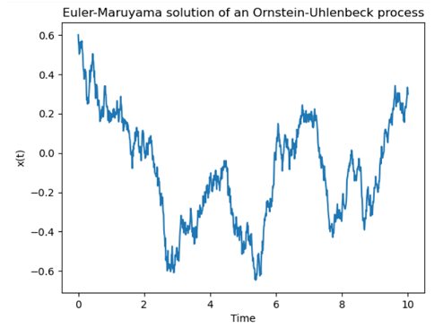


![\frac{\partial \rho(x, t)}{\partial t} = \gamma \frac{\partial}{\partial x} [x \rho(x, t)] + \frac{\sigma^2}{2}\frac{\partial^2 \rho(x, t)}{\partial x^2} \quad \quad \quad (2)](https://s0.wp.com/latex.php?latex=%5Cfrac%7B%5Cpartial+%5Crho%28x%2C+t%29%7D%7B%5Cpartial+t%7D+%3D+%5Cgamma+%5Cfrac%7B%5Cpartial%7D%7B%5Cpartial+x%7D+%5Bx+%5Crho%28x%2C+t%29%5D+%2B+%5Cfrac%7B%5Csigma%5E2%7D%7B2%7D%5Cfrac%7B%5Cpartial%5E2+%5Crho%28x%2C+t%29%7D%7B%5Cpartial+x%5E2%7D+%5Cquad+%5Cquad+%5Cquad+%282%29+&bg=ffffff&fg=111111&s=1&c=20201002)

![0 = \gamma \frac{\partial}{\partial x} [x \rho(x, t)] + \frac{\sigma^2}{2}\frac{\partial^2 \rho(x, t)}{\partial x^2}](https://s0.wp.com/latex.php?latex=0+%3D+%5Cgamma+%5Cfrac%7B%5Cpartial%7D%7B%5Cpartial+x%7D+%5Bx+%5Crho%28x%2C+t%29%5D+%2B+%5Cfrac%7B%5Csigma%5E2%7D%7B2%7D%5Cfrac%7B%5Cpartial%5E2+%5Crho%28x%2C+t%29%7D%7B%5Cpartial+x%5E2%7D+&bg=ffffff&fg=111111&s=1&c=20201002)
![= \frac{d}{d x} \bigg[\gamma x \rho(x) + \frac{\sigma^2}{2} \frac{d \rho(x)}{dx} \bigg] \quad \quad \quad \quad (3)](https://s0.wp.com/latex.php?latex=%3D+%5Cfrac%7Bd%7D%7Bd+x%7D+%5Cbigg%5B%5Cgamma+x+%5Crho%28x%29+%2B+%5Cfrac%7B%5Csigma%5E2%7D%7B2%7D+%5Cfrac%7Bd+%5Crho%28x%29%7D%7Bdx%7D+%5Cbigg%5D+%5Cquad+%5Cquad+%5Cquad+%5Cquad+%283%29+&bg=ffffff&fg=111111&s=1&c=20201002)


![= [y \exp(-y^2)]_{-\infty}^{\infty} - \int_{-\infty}^{\infty} y(-2y \exp(-y^2))dy](https://s0.wp.com/latex.php?latex=%3D+%5By+%5Cexp%28-y%5E2%29%5D_%7B-%5Cinfty%7D%5E%7B%5Cinfty%7D+-+%5Cint_%7B-%5Cinfty%7D%5E%7B%5Cinfty%7D+y%28-2y+%5Cexp%28-y%5E2%29%29dy+&bg=ffffff&fg=111111&s=1&c=20201002)


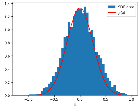
![[0, T]](https://s0.wp.com/latex.php?latex=%5B0%2C+T%5D&bg=ffffff&fg=111111&s=0&c=20201002) and we divide it into
and we divide it into 
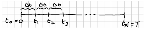
 , define the simple random walk
 we have
 are easily calculated as
![E[\Delta W_{n+1}] = \frac{1}{2} (\Delta h) + \frac{1}{2} (-\Delta h) = 0 \quad \quad \quad \quad (3)](https://s0.wp.com/latex.php?latex=E%5B%5CDelta+W_%7Bn%2B1%7D%5D+%3D+%5Cfrac%7B1%7D%7B2%7D+%28%5CDelta+h%29+%2B+%5Cfrac%7B1%7D%7B2%7D+%28-%5CDelta+h%29+%3D+0+%5Cquad+%5Cquad+%5Cquad+%5Cquad+%283%29+&bg=ffffff&fg=111111&s=1&c=20201002)
![V[\Delta W_{n+1}] = E[\Delta W_{n+1}^2] - E^2[\Delta W_{n+1}]](https://s0.wp.com/latex.php?latex=V%5B%5CDelta+W_%7Bn%2B1%7D%5D+%3D+E%5B%5CDelta+W_%7Bn%2B1%7D%5E2%5D+-+E%5E2%5B%5CDelta+W_%7Bn%2B1%7D%5D+&bg=ffffff&fg=111111&s=1&c=20201002)


 , as illustrated in the following picture:

 . The mean and variance of
  are again easily calculated as
![E[\Delta x_T] = \sum_{k=1}^{N} E[\Delta W_k] = 0 \quad \quad \quad \quad (6)](https://s0.wp.com/latex.php?latex=E%5B%5CDelta+x_T%5D+%3D+%5Csum_%7Bk%3D1%7D%5E%7BN%7D+E%5B%5CDelta+W_k%5D+%3D+0+%5Cquad+%5Cquad+%5Cquad+%5Cquad+%286%29+&bg=ffffff&fg=111111&s=1&c=20201002)
![V[\Delta x_T] = \sum_{k=1}^{N} V[\Delta W_k] = N(\Delta h)^2 = \frac{T}{\Delta t} (\Delta h)^2 \quad \quad \quad \quad (7)](https://s0.wp.com/latex.php?latex=V%5B%5CDelta+x_T%5D+%3D+%5Csum_%7Bk%3D1%7D%5E%7BN%7D+V%5B%5CDelta+W_k%5D+%3D+N%28%5CDelta+h%29%5E2+%3D+%5Cfrac%7BT%7D%7B%5CDelta+t%7D+%28%5CDelta+h%29%5E2+%5Cquad+%5Cquad+%5Cquad+%5Cquad+%287%29+&bg=ffffff&fg=111111&s=1&c=20201002)
 , it must be the case that
  . From (7) we then obtain
 ![V[x_T] = T \quad \quad \quad \quad (8)](https://s0.wp.com/latex.php?latex=V%5Bx_T%5D+%3D+T+%5Cquad+%5Cquad+%5Cquad+%5Cquad+%288%29+&bg=ffffff&fg=111111&s=1&c=20201002)
 would lead to the variance of the random walk either exploding (if
  ) or flatlining (if
  ), rather than settling into a Wiener process as
  to
to  , the simple random walk underlying the Wiener process can reach a point
  or by decreasing from the point
  , as illustrated in the following picture:
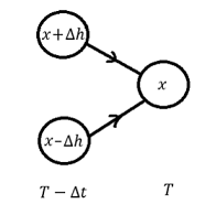
 we are looking for must satisfy
 to obtain


 and letting


 with
with  , the underlying random variable
  is one that counts the number of successes in the first
  of failure. The probability function for

 for
for  , where each indicator takes the value 1 meaning success with probability
![E[I_k] = p \quad \quad \quad \quad (4)](https://s0.wp.com/latex.php?latex=E%5BI_k%5D+%3D+p+%5Cquad+%5Cquad+%5Cquad+%5Cquad+%284%29+&bg=ffffff&fg=111111&s=1&c=20201002)
![V[I_k] = E[I_k^2] - E^2[I_k] = pq \quad \quad \quad \quad (5)](https://s0.wp.com/latex.php?latex=V%5BI_k%5D+%3D+E%5BI_k%5E2%5D+-+E%5E2%5BI_k%5D+%3D+pq+%5Cquad+%5Cquad+%5Cquad+%5Cquad+%285%29+&bg=ffffff&fg=111111&s=1&c=20201002)
![E[X] = Np \quad \quad \quad \quad (6)](https://s0.wp.com/latex.php?latex=E%5BX%5D+%3D+Np+%5Cquad+%5Cquad+%5Cquad+%5Cquad+%286%29+&bg=ffffff&fg=111111&s=1&c=20201002)
![V[X] = Npq \quad \quad \quad \quad (7)](https://s0.wp.com/latex.php?latex=V%5BX%5D+%3D+Npq+%5Cquad+%5Cquad+%5Cquad+%5Cquad+%287%29+&bg=ffffff&fg=111111&s=1&c=20201002)
![E[X]](https://s0.wp.com/latex.php?latex=E%5BX%5D&bg=ffffff&fg=111111&s=0&c=20201002) and
and ![E[X^2]](https://s0.wp.com/latex.php?latex=E%5BX%5E2%5D&bg=ffffff&fg=111111&s=0&c=20201002) using the probability functions in (1) above, i.e.,
using the probability functions in (1) above, i.e.,![E[X] = \sum_{n=0}^N n \cdot P(X = n)](https://s0.wp.com/latex.php?latex=E%5BX%5D+%3D+%5Csum_%7Bn%3D0%7D%5EN+n+%5Ccdot+P%28X+%3D+n%29+&bg=ffffff&fg=111111&s=1&c=20201002)

![E[X^2] = \sum_{n=0}^N n^2 \cdot P(X = n)](https://s0.wp.com/latex.php?latex=E%5BX%5E2%5D+%3D+%5Csum_%7Bn%3D0%7D%5EN+n%5E2+%5Ccdot+P%28X+%3D+n%29+&bg=ffffff&fg=111111&s=1&c=20201002)

 as follows:

![E[X] = \sum_{n=1}^N n \cdot C(N, n) p^n q^{N-n}](https://s0.wp.com/latex.php?latex=E%5BX%5D+%3D+%5Csum_%7Bn%3D1%7D%5EN+n+%5Ccdot+C%28N%2C+n%29+p%5En+q%5E%7BN-n%7D+&bg=ffffff&fg=111111&s=1&c=20201002)


 as follows:
![= [(n-1) + 1] \cdot \frac{(N-1)!}{(n-1)! (N-n)!}](https://s0.wp.com/latex.php?latex=%3D+%5B%28n-1%29+%2B+1%5D+%5Ccdot+%5Cfrac%7B%28N-1%29%21%7D%7B%28n-1%29%21+%28N-n%29%21%7D+&bg=ffffff&fg=111111&s=1&c=20201002)


![E[X^2] = \sum_{n=1}^N n^2 \cdot C(N, n) p^n q^{N-n}](https://s0.wp.com/latex.php?latex=E%5BX%5E2%5D+%3D+%5Csum_%7Bn%3D1%7D%5EN+n%5E2+%5Ccdot+C%28N%2C+n%29+p%5En+q%5E%7BN-n%7D+&bg=ffffff&fg=111111&s=1&c=20201002)


![V[X] = E[X^2] - E^2[X]](https://s0.wp.com/latex.php?latex=V%5BX%5D+%3D+E%5BX%5E2%5D+-+E%5E2%5BX%5D+&bg=ffffff&fg=111111&s=1&c=20201002)


 :
:

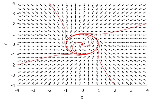

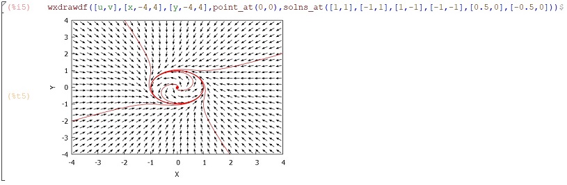


 and
and  are the coordinates of the first and second mass respectively. These equations differ from the standard case only in that the
  and the coordinate
  units, the coordinate
  units to maintain the equilibrium (e.g., to stop the spring being stretched). However, if the coordinate
  units, then the coordinate
  units to maintain the equilibrium. And so on. Whenever the position of the second mass is not exactly
 with corresponding eigenvectors
  and
and  . The first eigenvector shows that the masses will not move through space at the same speed, while the different signs of the components of the second eigenvector indicate that the corresponding normal mode of oscillations of the system at frequency
  is phase-opposed.


 with corresponding eigenvectors
  and
and  is phase-opposed.
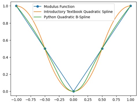
 of order
  as
as  if
if  , where
  is a strictly increasing sequence of breakpoints and
  is any sequence of polynomials of order
  ). At each breakpoint other than
  and
and  , the pp function is (arbitrarily) defined for computational purposes as taking the value from the right, i.e.,
  for
for  . The collection of all pp functions of order
  is a linear space of dimension
  denoted by
  .
.
 and
and  , where the notation means the jump of the function across the site
  , and
, and  is a set of nonnegative integers with
  counting the number of continuity conditions required at
  or
or  in this list as continuity conditions are only needed to govern how different pieces of the pp function `meet’ at interior breakpoints). For example,
  means that both the function and the first derivative are required to be continuous at
  means that there are no continuity conditions at
  satisfying the continuity conditions is a linear subspace of
  . The dimension of
 be a nondecreasing sequence of numbers (these are called `knots’ in the context of splines, and can be viewed as an extension of the breakpoint sequence
  -th normalised B-Spline of order
  ) using knot sequence
  , and its value at a site
  is given by
 , which is given by
 and has support
  , so it is continuous from the right in accordance with the convention for pp functions stated earlier. By putting
  which is a piecewise polynomial of order
  . B-Splines of higher order can be found via the recurrence relation in a convenient way using a tableau similar to the one commonly used to work out divided differences of functions.
 is a basis for
  for all
  ;
; is a nondecreasing sequence with
  ;
; times in
  and
and  .
. times, the function and its first derivative are continuous at
 so the parameter
 (corresponding to a degree
  for the polynomial pieces), and there are two continuity conditions for each of the interior points in the breakpoint sequence (the function and its first derivative are continuous) so using the standard notation we have
  . The dimension of the subspace is thus
  so we expect to have five B-Splines in the basis set. In the picture below, I plot on the left the five basis B-Splines corresponding to

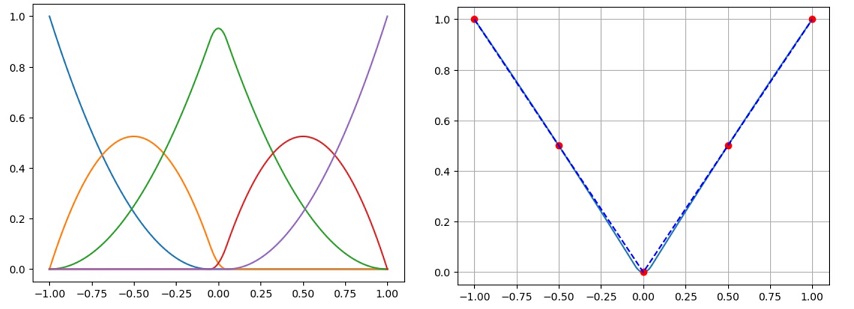
 in the form
 is the highest value of
  or
or  is non-zero, i.e.,
![q(x) = \frac{1}{2}a_0 + \sum_{j=1}^n\big[a_j \cos(jx) + b_j \sin(jx) \big]](https://s0.wp.com/latex.php?latex=q%28x%29+%3D+%5Cfrac%7B1%7D%7B2%7Da_0+%2B+%5Csum_%7Bj%3D1%7D%5En%5Cbig%5Ba_j+%5Ccos%28jx%29+%2B+b_j+%5Csin%28jx%29+%5Cbig%5D&bg=ffffff&fg=111111&s=0&c=20201002)
 as a trigonometric polynomial of degree
  ,
,  and
and  respectively:


 in the Fourier series expansion of
  term by term. We get
 or of
or of  and
and  (i.e.,
  ). We are thus left with
 , we multiply both sides of the generic Fourier series expansion by
  and again find the average value of each term to get
 and take average values. We find
![[-\pi, \pi]](https://s0.wp.com/latex.php?latex=%5B-%5Cpi%2C+%5Cpi%5D&bg=ffffff&fg=111111&s=0&c=20201002) . When this is not the case and we only have the values of
. When this is not the case and we only have the values of 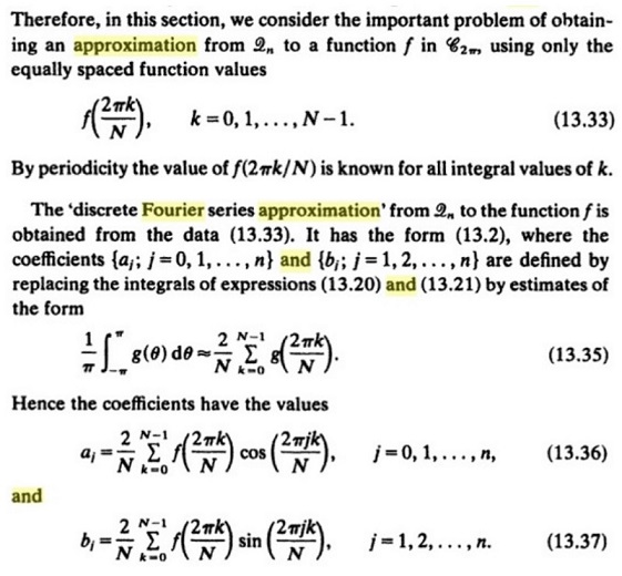
 ,
,  ,
,  and
and  . Thus, we need to obtain an approximation to
 ![q(x) = \frac{1}{2}a_0 + \sum_{j=1}^2\big[a_j \cos(jx) + b_j \sin(jx) \big]](https://s0.wp.com/latex.php?latex=q%28x%29+%3D+%5Cfrac%7B1%7D%7B2%7Da_0+%2B+%5Csum_%7Bj%3D1%7D%5E2%5Cbig%5Ba_j+%5Ccos%28jx%29+%2B+b_j+%5Csin%28jx%29+%5Cbig%5D&bg=ffffff&fg=111111&s=0&c=20201002)
 , we use formulas (13.36) and (13.37) to evaluate the coefficients
  ,
,  ,
,  and
and  as follows:
![= \frac{2}{4} \big[f(0)\cos(0) + f\big(\frac{2\pi}{4}\big) + f\big(\frac{4\pi}{4}\big) + f\big(\frac{6\pi}{4}\big)\big] = 0.975](https://s0.wp.com/latex.php?latex=%3D+%5Cfrac%7B2%7D%7B4%7D+%5Cbig%5Bf%280%29%5Ccos%280%29+%2B+f%5Cbig%28%5Cfrac%7B2%5Cpi%7D%7B4%7D%5Cbig%29+%2B+f%5Cbig%28%5Cfrac%7B4%5Cpi%7D%7B4%7D%5Cbig%29+%2B+f%5Cbig%28%5Cfrac%7B6%5Cpi%7D%7B4%7D%5Cbig%29%5Cbig%5D+%3D+0.975&bg=ffffff&fg=111111&s=0&c=20201002)
![a_1 = \frac{2}{4} \big[f(0)\cos(0) + f\big(\frac{2\pi}{4}\big)\cos\big(\frac{2\pi}{4}\big) + f\big(\frac{4\pi}{4}\big)\cos\big(\frac{4\pi}{4}\big) + f\big(\frac{6\pi}{4}\big)\cos\big(\frac{6\pi}{4}\big)\big] = -0.4](https://s0.wp.com/latex.php?latex=a_1+%3D+%5Cfrac%7B2%7D%7B4%7D+%5Cbig%5Bf%280%29%5Ccos%280%29+%2B+f%5Cbig%28%5Cfrac%7B2%5Cpi%7D%7B4%7D%5Cbig%29%5Ccos%5Cbig%28%5Cfrac%7B2%5Cpi%7D%7B4%7D%5Cbig%29+%2B+f%5Cbig%28%5Cfrac%7B4%5Cpi%7D%7B4%7D%5Cbig%29%5Ccos%5Cbig%28%5Cfrac%7B4%5Cpi%7D%7B4%7D%5Cbig%29+%2B+f%5Cbig%28%5Cfrac%7B6%5Cpi%7D%7B4%7D%5Cbig%29%5Ccos%5Cbig%28%5Cfrac%7B6%5Cpi%7D%7B4%7D%5Cbig%29%5Cbig%5D+%3D+-0.4&bg=ffffff&fg=111111&s=0&c=20201002)
![a_2 = \frac{2}{4} \big[f(0)\cos(0) + f\big(\frac{2\pi}{4}\big)\cos\big(\frac{4\pi}{4}\big) + f\big(\frac{4\pi}{4}\big)\cos\big(\frac{8\pi}{4}\big) + f\big(\frac{6\pi}{4}\big)\cos\big(\frac{12\pi}{4}\big)\big] = 0.225](https://s0.wp.com/latex.php?latex=a_2+%3D+%5Cfrac%7B2%7D%7B4%7D+%5Cbig%5Bf%280%29%5Ccos%280%29+%2B+f%5Cbig%28%5Cfrac%7B2%5Cpi%7D%7B4%7D%5Cbig%29%5Ccos%5Cbig%28%5Cfrac%7B4%5Cpi%7D%7B4%7D%5Cbig%29+%2B+f%5Cbig%28%5Cfrac%7B4%5Cpi%7D%7B4%7D%5Cbig%29%5Ccos%5Cbig%28%5Cfrac%7B8%5Cpi%7D%7B4%7D%5Cbig%29+%2B+f%5Cbig%28%5Cfrac%7B6%5Cpi%7D%7B4%7D%5Cbig%29%5Ccos%5Cbig%28%5Cfrac%7B12%5Cpi%7D%7B4%7D%5Cbig%29%5Cbig%5D+%3D+0.225&bg=ffffff&fg=111111&s=0&c=20201002)

![= \frac{2}{4} \big[f(0)\sin(0) + f\big(\frac{2\pi}{4}\big)\sin\big(\frac{2\pi}{4}\big) + f\big(\frac{4\pi}{4}\big)\sin\big(\frac{4\pi}{4}\big) + f\big(\frac{6\pi}{4}\big)\sin\big(\frac{6\pi}{4}\big)\big] = -0.125](https://s0.wp.com/latex.php?latex=%3D+%5Cfrac%7B2%7D%7B4%7D+%5Cbig%5Bf%280%29%5Csin%280%29+%2B+f%5Cbig%28%5Cfrac%7B2%5Cpi%7D%7B4%7D%5Cbig%29%5Csin%5Cbig%28%5Cfrac%7B2%5Cpi%7D%7B4%7D%5Cbig%29+%2B+f%5Cbig%28%5Cfrac%7B4%5Cpi%7D%7B4%7D%5Cbig%29%5Csin%5Cbig%28%5Cfrac%7B4%5Cpi%7D%7B4%7D%5Cbig%29+%2B+f%5Cbig%28%5Cfrac%7B6%5Cpi%7D%7B4%7D%5Cbig%29%5Csin%5Cbig%28%5Cfrac%7B6%5Cpi%7D%7B4%7D%5Cbig%29%5Cbig%5D+%3D+-0.125&bg=ffffff&fg=111111&s=0&c=20201002)
![b_2 = \frac{2}{4} \big[f(0)\sin(0) + f\big(\frac{2\pi}{4}\big)\sin\big(\frac{4\pi}{4}\big) + f\big(\frac{4\pi}{4}\big)\sin\big(\frac{8\pi}{4}\big) + f\big(\frac{6\pi}{4}\big)\sin\big(\frac{12\pi}{4}\big)\big] = 0](https://s0.wp.com/latex.php?latex=b_2+%3D+%5Cfrac%7B2%7D%7B4%7D+%5Cbig%5Bf%280%29%5Csin%280%29+%2B+f%5Cbig%28%5Cfrac%7B2%5Cpi%7D%7B4%7D%5Cbig%29%5Csin%5Cbig%28%5Cfrac%7B4%5Cpi%7D%7B4%7D%5Cbig%29+%2B+f%5Cbig%28%5Cfrac%7B4%5Cpi%7D%7B4%7D%5Cbig%29%5Csin%5Cbig%28%5Cfrac%7B8%5Cpi%7D%7B4%7D%5Cbig%29+%2B+f%5Cbig%28%5Cfrac%7B6%5Cpi%7D%7B4%7D%5Cbig%29%5Csin%5Cbig%28%5Cfrac%7B12%5Cpi%7D%7B4%7D%5Cbig%29%5Cbig%5D+%3D+0&bg=ffffff&fg=111111&s=0&c=20201002)


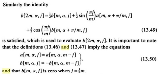
 , in the third iteration we have
  , in the fourth iteration we have
  and so on. This continues until the value of the iteration variable reaches
  and
and ![a[1, \alpha, 0] = 2f(\alpha)](https://s0.wp.com/latex.php?latex=a%5B1%2C+%5Calpha%2C+0%5D+%3D+2f%28%5Calpha%29&bg=ffffff&fg=111111&s=0&c=20201002)
![b[1, \alpha, 0] = 0](https://s0.wp.com/latex.php?latex=b%5B1%2C+%5Calpha%2C+0%5D+%3D+0&bg=ffffff&fg=111111&s=0&c=20201002)

![a[1, \alpha, 0]](https://s0.wp.com/latex.php?latex=a%5B1%2C+%5Calpha%2C+0%5D&bg=ffffff&fg=111111&s=0&c=20201002) and
and ![b[1, \alpha, 0]](https://s0.wp.com/latex.php?latex=b%5B1%2C+%5Calpha%2C+0%5D&bg=ffffff&fg=111111&s=0&c=20201002) . We then use formulas (13.50) to obtain the numbers
. We then use formulas (13.50) to obtain the numbers ![a[1, \alpha, 1]](https://s0.wp.com/latex.php?latex=a%5B1%2C+%5Calpha%2C+1%5D&bg=ffffff&fg=111111&s=0&c=20201002) and
and ![b[1, \alpha, 1]](https://s0.wp.com/latex.php?latex=b%5B1%2C+%5Calpha%2C+1%5D&bg=ffffff&fg=111111&s=0&c=20201002) . We get
. We get![a[1, \alpha, 1] = a[1, \alpha, 0] = 2f(\alpha)](https://s0.wp.com/latex.php?latex=a%5B1%2C+%5Calpha%2C+1%5D+%3D+a%5B1%2C+%5Calpha%2C+0%5D+%3D+2f%28%5Calpha%29&bg=ffffff&fg=111111&s=0&c=20201002)
![b[1, \alpha, 1] = -b[1, \alpha, 0] = 0](https://s0.wp.com/latex.php?latex=b%5B1%2C+%5Calpha%2C+1%5D+%3D+-b%5B1%2C+%5Calpha%2C+0%5D+%3D+0&bg=ffffff&fg=111111&s=0&c=20201002)
![a[2, \alpha, j]](https://s0.wp.com/latex.php?latex=a%5B2%2C+%5Calpha%2C+j%5D&bg=ffffff&fg=111111&s=0&c=20201002) and
and ![b[2, \alpha, j]](https://s0.wp.com/latex.php?latex=b%5B2%2C+%5Calpha%2C+j%5D&bg=ffffff&fg=111111&s=0&c=20201002) for
for  using formulas (13.48) and (13.49). The variable
  in this second iteration. We then use formulas (13.50) to obtain the numbers
  and at this point we are ready to begin the third iteration.
![a[4, \alpha, j]](https://s0.wp.com/latex.php?latex=a%5B4%2C+%5Calpha%2C+j%5D&bg=ffffff&fg=111111&s=0&c=20201002) and
and ![b[4, \alpha, j]](https://s0.wp.com/latex.php?latex=b%5B4%2C+%5Calpha%2C+j%5D&bg=ffffff&fg=111111&s=0&c=20201002) for
for  using formulas (13.48) and (13.49). The variable
  in this third iteration. We then use formulas (13.50) to obtain the numbers
  and at this point we are ready to begin the fourth iteration.
![a[8, \alpha, j]](https://s0.wp.com/latex.php?latex=a%5B8%2C+%5Calpha%2C+j%5D&bg=ffffff&fg=111111&s=0&c=20201002) and
and ![b[8, \alpha, j]](https://s0.wp.com/latex.php?latex=b%5B8%2C+%5Calpha%2C+j%5D&bg=ffffff&fg=111111&s=0&c=20201002) for
for  using formulas (13.48) and (13.49). The variable
  in this fourth iteration. We then use formulas (13.50) to obtain the numbers
  and at this point we are ready to begin the fifth iteration.
![a[m, \alpha, j]](https://s0.wp.com/latex.php?latex=a%5Bm%2C+%5Calpha%2C+j%5D&bg=ffffff&fg=111111&s=0&c=20201002) and
and ![b[m, \alpha, j]](https://s0.wp.com/latex.php?latex=b%5Bm%2C+%5Calpha%2C+j%5D&bg=ffffff&fg=111111&s=0&c=20201002) are known, where
are known, where ![[0, m]](https://s0.wp.com/latex.php?latex=%5B0%2C+m%5D&bg=ffffff&fg=111111&s=0&c=20201002) and the variable
and the variable  . The iterations continue in this fashion until we arrive at the numbers
 ![a_j = a[N, 0, j]](https://s0.wp.com/latex.php?latex=a_j+%3D+a%5BN%2C+0%2C+j%5D&bg=ffffff&fg=111111&s=0&c=20201002) and
and ![b_j = b[N, 0, j]](https://s0.wp.com/latex.php?latex=b_j+%3D+b%5BN%2C+0%2C+j%5D&bg=ffffff&fg=111111&s=0&c=20201002) for
for  and these provide the required coefficients for the approximation.
![q(x) = \frac{1}{2}a_0 + \sum_{j=1}^3\big[a_j \cos(jx) + b_j \sin(jx) \big]](https://s0.wp.com/latex.php?latex=q%28x%29+%3D+%5Cfrac%7B1%7D%7B2%7Da_0+%2B+%5Csum_%7Bj%3D1%7D%5E3%5Cbig%5Ba_j+%5Ccos%28jx%29+%2B+b_j+%5Csin%28jx%29+%5Cbig%5D&bg=ffffff&fg=111111&s=0&c=20201002)
 , we begin by setting
  in formulas (13.46) and (13.47). Formula (13.46) reduces to
![a\big[1, \frac{2\pi \cdot 0}{8}, 0\big] = 2f\big(\frac{2\pi \cdot 0}{8}\big) = -0.224356](https://s0.wp.com/latex.php?latex=a%5Cbig%5B1%2C+%5Cfrac%7B2%5Cpi+%5Ccdot+0%7D%7B8%7D%2C+0%5Cbig%5D+%3D+2f%5Cbig%28%5Cfrac%7B2%5Cpi+%5Ccdot+0%7D%7B8%7D%5Cbig%29+%3D+-0.224356&bg=ffffff&fg=111111&s=0&c=20201002)
![a\big[1, \frac{2\pi \cdot 1}{8}, 0\big] = 2f\big(\frac{2\pi \cdot 1}{8}\big) = 2.159318](https://s0.wp.com/latex.php?latex=a%5Cbig%5B1%2C+%5Cfrac%7B2%5Cpi+%5Ccdot+1%7D%7B8%7D%2C+0%5Cbig%5D+%3D+2f%5Cbig%28%5Cfrac%7B2%5Cpi+%5Ccdot+1%7D%7B8%7D%5Cbig%29+%3D+2.159318&bg=ffffff&fg=111111&s=0&c=20201002)
![a\big[1, \frac{2\pi \cdot 2}{8}, 0\big] = 2f\big(\frac{2\pi \cdot 2}{8}\big) = 4.345334](https://s0.wp.com/latex.php?latex=a%5Cbig%5B1%2C+%5Cfrac%7B2%5Cpi+%5Ccdot+2%7D%7B8%7D%2C+0%5Cbig%5D+%3D+2f%5Cbig%28%5Cfrac%7B2%5Cpi+%5Ccdot+2%7D%7B8%7D%5Cbig%29+%3D+4.345334&bg=ffffff&fg=111111&s=0&c=20201002)
![a\big[1, \frac{2\pi \cdot 3}{8}, 0\big] = 2f\big(\frac{2\pi \cdot 3}{8}\big) = 0.753214](https://s0.wp.com/latex.php?latex=a%5Cbig%5B1%2C+%5Cfrac%7B2%5Cpi+%5Ccdot+3%7D%7B8%7D%2C+0%5Cbig%5D+%3D+2f%5Cbig%28%5Cfrac%7B2%5Cpi+%5Ccdot+3%7D%7B8%7D%5Cbig%29+%3D+0.753214&bg=ffffff&fg=111111&s=0&c=20201002)
![a\big[1, \frac{2\pi \cdot 4}{8}, 0\big] = 2f\big(\frac{2\pi \cdot 4}{8}\big) = -0.642824](https://s0.wp.com/latex.php?latex=a%5Cbig%5B1%2C+%5Cfrac%7B2%5Cpi+%5Ccdot+4%7D%7B8%7D%2C+0%5Cbig%5D+%3D+2f%5Cbig%28%5Cfrac%7B2%5Cpi+%5Ccdot+4%7D%7B8%7D%5Cbig%29+%3D+-0.642824&bg=ffffff&fg=111111&s=0&c=20201002)
![a\big[1, \frac{2\pi \cdot 5}{8}, 0\big] = 2f\big(\frac{2\pi \cdot 5}{8}\big) = -1.056226](https://s0.wp.com/latex.php?latex=a%5Cbig%5B1%2C+%5Cfrac%7B2%5Cpi+%5Ccdot+5%7D%7B8%7D%2C+0%5Cbig%5D+%3D+2f%5Cbig%28%5Cfrac%7B2%5Cpi+%5Ccdot+5%7D%7B8%7D%5Cbig%29+%3D+-1.056226&bg=ffffff&fg=111111&s=0&c=20201002)
![a\big[1, \frac{2\pi \cdot 6}{8}, 0\big] = 2f\big(\frac{2\pi \cdot 6}{8}\big) = -1.124652](https://s0.wp.com/latex.php?latex=a%5Cbig%5B1%2C+%5Cfrac%7B2%5Cpi+%5Ccdot+6%7D%7B8%7D%2C+0%5Cbig%5D+%3D+2f%5Cbig%28%5Cfrac%7B2%5Cpi+%5Ccdot+6%7D%7B8%7D%5Cbig%29+%3D+-1.124652&bg=ffffff&fg=111111&s=0&c=20201002)
![a\big[1, \frac{2\pi \cdot 7}{8}, 0\big] = 2f\big(\frac{2\pi \cdot 7}{8}\big) = -0.932522](https://s0.wp.com/latex.php?latex=a%5Cbig%5B1%2C+%5Cfrac%7B2%5Cpi+%5Ccdot+7%7D%7B8%7D%2C+0%5Cbig%5D+%3D+2f%5Cbig%28%5Cfrac%7B2%5Cpi+%5Ccdot+7%7D%7B8%7D%5Cbig%29+%3D+-0.932522&bg=ffffff&fg=111111&s=0&c=20201002)
![b\big[1, \frac{2\pi \cdot 0}{8}, 0\big] = 0](https://s0.wp.com/latex.php?latex=b%5Cbig%5B1%2C+%5Cfrac%7B2%5Cpi+%5Ccdot+0%7D%7B8%7D%2C+0%5Cbig%5D+%3D+0&bg=ffffff&fg=111111&s=0&c=20201002)
![b\big[1, \frac{2\pi \cdot 1}{8}, 0\big] = 0](https://s0.wp.com/latex.php?latex=b%5Cbig%5B1%2C+%5Cfrac%7B2%5Cpi+%5Ccdot+1%7D%7B8%7D%2C+0%5Cbig%5D+%3D+0&bg=ffffff&fg=111111&s=0&c=20201002)
![b\big[1, \frac{2\pi \cdot 2}{8}, 0\big] = 0](https://s0.wp.com/latex.php?latex=b%5Cbig%5B1%2C+%5Cfrac%7B2%5Cpi+%5Ccdot+2%7D%7B8%7D%2C+0%5Cbig%5D+%3D+0&bg=ffffff&fg=111111&s=0&c=20201002)
![b\big[1, \frac{2\pi \cdot 3}{8}, 0\big] = 0](https://s0.wp.com/latex.php?latex=b%5Cbig%5B1%2C+%5Cfrac%7B2%5Cpi+%5Ccdot+3%7D%7B8%7D%2C+0%5Cbig%5D+%3D+0&bg=ffffff&fg=111111&s=0&c=20201002)
![b\big[1, \frac{2\pi \cdot 4}{8}, 0\big] = 0](https://s0.wp.com/latex.php?latex=b%5Cbig%5B1%2C+%5Cfrac%7B2%5Cpi+%5Ccdot+4%7D%7B8%7D%2C+0%5Cbig%5D+%3D+0&bg=ffffff&fg=111111&s=0&c=20201002)
![b\big[1, \frac{2\pi \cdot 5}{8}, 0\big] = 0](https://s0.wp.com/latex.php?latex=b%5Cbig%5B1%2C+%5Cfrac%7B2%5Cpi+%5Ccdot+5%7D%7B8%7D%2C+0%5Cbig%5D+%3D+0&bg=ffffff&fg=111111&s=0&c=20201002)
![b\big[1, \frac{2\pi \cdot 6}{8}, 0\big] = 0](https://s0.wp.com/latex.php?latex=b%5Cbig%5B1%2C+%5Cfrac%7B2%5Cpi+%5Ccdot+6%7D%7B8%7D%2C+0%5Cbig%5D+%3D+0&bg=ffffff&fg=111111&s=0&c=20201002)
![b\big[1, \frac{2\pi \cdot 7}{8}, 0\big] = 0](https://s0.wp.com/latex.php?latex=b%5Cbig%5B1%2C+%5Cfrac%7B2%5Cpi+%5Ccdot+7%7D%7B8%7D%2C+0%5Cbig%5D+%3D+0&bg=ffffff&fg=111111&s=0&c=20201002)
![a\big[1, \frac{2\pi \cdot 0}{8}, 1\big] = -0.224356](https://s0.wp.com/latex.php?latex=a%5Cbig%5B1%2C+%5Cfrac%7B2%5Cpi+%5Ccdot+0%7D%7B8%7D%2C+1%5Cbig%5D+%3D+-0.224356&bg=ffffff&fg=111111&s=0&c=20201002)
![a\big[1, \frac{2\pi \cdot 1}{8}, 1\big] = 2.159318](https://s0.wp.com/latex.php?latex=a%5Cbig%5B1%2C+%5Cfrac%7B2%5Cpi+%5Ccdot+1%7D%7B8%7D%2C+1%5Cbig%5D+%3D+2.159318&bg=ffffff&fg=111111&s=0&c=20201002)
![a\big[1, \frac{2\pi \cdot 2}{8}, 1\big] = 4.345334](https://s0.wp.com/latex.php?latex=a%5Cbig%5B1%2C+%5Cfrac%7B2%5Cpi+%5Ccdot+2%7D%7B8%7D%2C+1%5Cbig%5D+%3D+4.345334&bg=ffffff&fg=111111&s=0&c=20201002)
![a\big[1, \frac{2\pi \cdot 3}{8}, 1\big] = 0.753214](https://s0.wp.com/latex.php?latex=a%5Cbig%5B1%2C+%5Cfrac%7B2%5Cpi+%5Ccdot+3%7D%7B8%7D%2C+1%5Cbig%5D+%3D+0.753214&bg=ffffff&fg=111111&s=0&c=20201002)
![a\big[1, \frac{2\pi \cdot 4}{8}, 1\big] = -0.642824](https://s0.wp.com/latex.php?latex=a%5Cbig%5B1%2C+%5Cfrac%7B2%5Cpi+%5Ccdot+4%7D%7B8%7D%2C+1%5Cbig%5D+%3D+-0.642824&bg=ffffff&fg=111111&s=0&c=20201002)
![a\big[1, \frac{2\pi \cdot 5}{8}, 1\big] = -1.056226](https://s0.wp.com/latex.php?latex=a%5Cbig%5B1%2C+%5Cfrac%7B2%5Cpi+%5Ccdot+5%7D%7B8%7D%2C+1%5Cbig%5D+%3D+-1.056226&bg=ffffff&fg=111111&s=0&c=20201002)
![a\big[1, \frac{2\pi \cdot 6}{8}, 1\big] = -1.124652](https://s0.wp.com/latex.php?latex=a%5Cbig%5B1%2C+%5Cfrac%7B2%5Cpi+%5Ccdot+6%7D%7B8%7D%2C+1%5Cbig%5D+%3D+-1.124652&bg=ffffff&fg=111111&s=0&c=20201002)
![a\big[1, \frac{2\pi \cdot 7}{8}, 1\big] = -0.932522](https://s0.wp.com/latex.php?latex=a%5Cbig%5B1%2C+%5Cfrac%7B2%5Cpi+%5Ccdot+7%7D%7B8%7D%2C+1%5Cbig%5D+%3D+-0.932522&bg=ffffff&fg=111111&s=0&c=20201002)
![b\big[1, \frac{2\pi \cdot 0}{8}, 1\big] = 0](https://s0.wp.com/latex.php?latex=b%5Cbig%5B1%2C+%5Cfrac%7B2%5Cpi+%5Ccdot+0%7D%7B8%7D%2C+1%5Cbig%5D+%3D+0&bg=ffffff&fg=111111&s=0&c=20201002)
![b\big[1, \frac{2\pi \cdot 1}{8}, 1\big] = 0](https://s0.wp.com/latex.php?latex=b%5Cbig%5B1%2C+%5Cfrac%7B2%5Cpi+%5Ccdot+1%7D%7B8%7D%2C+1%5Cbig%5D+%3D+0&bg=ffffff&fg=111111&s=0&c=20201002)
![b\big[1, \frac{2\pi \cdot 2}{8}, 1\big] = 0](https://s0.wp.com/latex.php?latex=b%5Cbig%5B1%2C+%5Cfrac%7B2%5Cpi+%5Ccdot+2%7D%7B8%7D%2C+1%5Cbig%5D+%3D+0&bg=ffffff&fg=111111&s=0&c=20201002)
![b\big[1, \frac{2\pi \cdot 3}{8}, 1\big] = 0](https://s0.wp.com/latex.php?latex=b%5Cbig%5B1%2C+%5Cfrac%7B2%5Cpi+%5Ccdot+3%7D%7B8%7D%2C+1%5Cbig%5D+%3D+0&bg=ffffff&fg=111111&s=0&c=20201002)
![b\big[1, \frac{2\pi \cdot 4}{8}, 1\big] = 0](https://s0.wp.com/latex.php?latex=b%5Cbig%5B1%2C+%5Cfrac%7B2%5Cpi+%5Ccdot+4%7D%7B8%7D%2C+1%5Cbig%5D+%3D+0&bg=ffffff&fg=111111&s=0&c=20201002)
![b\big[1, \frac{2\pi \cdot 5}{8}, 1\big] = 0](https://s0.wp.com/latex.php?latex=b%5Cbig%5B1%2C+%5Cfrac%7B2%5Cpi+%5Ccdot+5%7D%7B8%7D%2C+1%5Cbig%5D+%3D+0&bg=ffffff&fg=111111&s=0&c=20201002)
![b\big[1, \frac{2\pi \cdot 6}{8}, 1\big] = 0](https://s0.wp.com/latex.php?latex=b%5Cbig%5B1%2C+%5Cfrac%7B2%5Cpi+%5Ccdot+6%7D%7B8%7D%2C+1%5Cbig%5D+%3D+0&bg=ffffff&fg=111111&s=0&c=20201002)
![b\big[1, \frac{2\pi \cdot 7}{8}, 1\big] = 0](https://s0.wp.com/latex.php?latex=b%5Cbig%5B1%2C+%5Cfrac%7B2%5Cpi+%5Ccdot+7%7D%7B8%7D%2C+1%5Cbig%5D+%3D+0&bg=ffffff&fg=111111&s=0&c=20201002)

 . We compute the numbers
 ![a[2, \alpha, 0]](https://s0.wp.com/latex.php?latex=a%5B2%2C+%5Calpha%2C+0%5D&bg=ffffff&fg=111111&s=0&c=20201002) ,
, ![a[2, \alpha, 1]](https://s0.wp.com/latex.php?latex=a%5B2%2C+%5Calpha%2C+1%5D&bg=ffffff&fg=111111&s=0&c=20201002) ,
, ![b[2, \alpha, 0]](https://s0.wp.com/latex.php?latex=b%5B2%2C+%5Calpha%2C+0%5D&bg=ffffff&fg=111111&s=0&c=20201002) and
and ![b[2, \alpha, 1]](https://s0.wp.com/latex.php?latex=b%5B2%2C+%5Calpha%2C+1%5D&bg=ffffff&fg=111111&s=0&c=20201002) using formulas (13.48) and (13.49). We get the formulas
using formulas (13.48) and (13.49). We get the formulas![a[2, \alpha, 0] = \frac{1}{2}\big\{a[1, \alpha, 0] + \cos(\pi \cdot 0/1)a[1, \alpha + \frac{\pi}{1}, 0] - \sin(\pi \cdot 0/1)b[1, \alpha + \frac{\pi}{1}, 0]\big\}](https://s0.wp.com/latex.php?latex=a%5B2%2C+%5Calpha%2C+0%5D+%3D+%5Cfrac%7B1%7D%7B2%7D%5Cbig%5C%7Ba%5B1%2C+%5Calpha%2C+0%5D+%2B+%5Ccos%28%5Cpi+%5Ccdot+0%2F1%29a%5B1%2C+%5Calpha+%2B+%5Cfrac%7B%5Cpi%7D%7B1%7D%2C+0%5D+-+%5Csin%28%5Cpi+%5Ccdot+0%2F1%29b%5B1%2C+%5Calpha+%2B+%5Cfrac%7B%5Cpi%7D%7B1%7D%2C+0%5D%5Cbig%5C%7D&bg=ffffff&fg=111111&s=0&c=20201002)
![= \frac{1}{2}\big\{a[1, \frac{2\pi \cdot k}{8}, 0] + a[1, \frac{2\pi}{8}(k + 4), 0]\big\}](https://s0.wp.com/latex.php?latex=%3D+%5Cfrac%7B1%7D%7B2%7D%5Cbig%5C%7Ba%5B1%2C+%5Cfrac%7B2%5Cpi+%5Ccdot+k%7D%7B8%7D%2C+0%5D+%2B+a%5B1%2C+%5Cfrac%7B2%5Cpi%7D%7B8%7D%28k+%2B+4%29%2C+0%5D%5Cbig%5C%7D&bg=ffffff&fg=111111&s=0&c=20201002)
![a[2, \alpha, 1] = \frac{1}{2}\big\{a[1, \alpha, 1] + \cos(\pi \cdot 1/1)a[1, \alpha + \frac{\pi}{1}, 1] - \sin(\pi \cdot 1/1)b[1, \alpha + \frac{\pi}{1}, 1]\big\}](https://s0.wp.com/latex.php?latex=a%5B2%2C+%5Calpha%2C+1%5D+%3D+%5Cfrac%7B1%7D%7B2%7D%5Cbig%5C%7Ba%5B1%2C+%5Calpha%2C+1%5D+%2B+%5Ccos%28%5Cpi+%5Ccdot+1%2F1%29a%5B1%2C+%5Calpha+%2B+%5Cfrac%7B%5Cpi%7D%7B1%7D%2C+1%5D+-+%5Csin%28%5Cpi+%5Ccdot+1%2F1%29b%5B1%2C+%5Calpha+%2B+%5Cfrac%7B%5Cpi%7D%7B1%7D%2C+1%5D%5Cbig%5C%7D&bg=ffffff&fg=111111&s=0&c=20201002)
![= \frac{1}{2}\big\{a[1, \frac{2\pi \cdot k}{8}, 1] - a[1, \frac{2\pi}{8}(k + 4), 1]\big\}](https://s0.wp.com/latex.php?latex=%3D+%5Cfrac%7B1%7D%7B2%7D%5Cbig%5C%7Ba%5B1%2C+%5Cfrac%7B2%5Cpi+%5Ccdot+k%7D%7B8%7D%2C+1%5D+-+a%5B1%2C+%5Cfrac%7B2%5Cpi%7D%7B8%7D%28k+%2B+4%29%2C+1%5D%5Cbig%5C%7D&bg=ffffff&fg=111111&s=0&c=20201002)
![b[2, \alpha, 0] = \frac{1}{2}\big\{b[1, \alpha, 0] + \sin(\pi \cdot 0/1)a[1, \alpha + \frac{\pi}{1}, 0] + \cos(\pi \cdot 0/1)b[1, \alpha + \frac{\pi}{1}, 0]\big\} = 0](https://s0.wp.com/latex.php?latex=b%5B2%2C+%5Calpha%2C+0%5D+%3D+%5Cfrac%7B1%7D%7B2%7D%5Cbig%5C%7Bb%5B1%2C+%5Calpha%2C+0%5D+%2B+%5Csin%28%5Cpi+%5Ccdot+0%2F1%29a%5B1%2C+%5Calpha+%2B+%5Cfrac%7B%5Cpi%7D%7B1%7D%2C+0%5D+%2B+%5Ccos%28%5Cpi+%5Ccdot+0%2F1%29b%5B1%2C+%5Calpha+%2B+%5Cfrac%7B%5Cpi%7D%7B1%7D%2C+0%5D%5Cbig%5C%7D+%3D+0&bg=ffffff&fg=111111&s=0&c=20201002)
![b[2, \alpha, 1] = \frac{1}{2}\big\{b[1, \alpha, 1] + \sin(\pi \cdot 1/1)a[1, \alpha + \frac{\pi}{1}, 1] + \cos(\pi \cdot 1/1)b[1, \alpha + \frac{\pi}{1}, 1]\big\} = 0](https://s0.wp.com/latex.php?latex=b%5B2%2C+%5Calpha%2C+1%5D+%3D+%5Cfrac%7B1%7D%7B2%7D%5Cbig%5C%7Bb%5B1%2C+%5Calpha%2C+1%5D+%2B+%5Csin%28%5Cpi+%5Ccdot+1%2F1%29a%5B1%2C+%5Calpha+%2B+%5Cfrac%7B%5Cpi%7D%7B1%7D%2C+1%5D+%2B+%5Ccos%28%5Cpi+%5Ccdot+1%2F1%29b%5B1%2C+%5Calpha+%2B+%5Cfrac%7B%5Cpi%7D%7B1%7D%2C+1%5D%5Cbig%5C%7D+%3D+0&bg=ffffff&fg=111111&s=0&c=20201002)
![a[2, \frac{2\pi \cdot 0}{8}, 0] = \frac{1}{2}\big\{a[1, \frac{2\pi \cdot 0}{8}, 0] + a[1, \frac{2\pi}{8}(0+ 4), 0]\big\}](https://s0.wp.com/latex.php?latex=a%5B2%2C+%5Cfrac%7B2%5Cpi+%5Ccdot+0%7D%7B8%7D%2C+0%5D+%3D+%5Cfrac%7B1%7D%7B2%7D%5Cbig%5C%7Ba%5B1%2C+%5Cfrac%7B2%5Cpi+%5Ccdot+0%7D%7B8%7D%2C+0%5D+%2B+a%5B1%2C+%5Cfrac%7B2%5Cpi%7D%7B8%7D%280%2B+4%29%2C+0%5D%5Cbig%5C%7D&bg=ffffff&fg=111111&s=0&c=20201002)

![a[2, \frac{2\pi \cdot 1}{8}, 0] = \frac{1}{2}\big\{a[1, \frac{2\pi \cdot 1}{8}, 0] + a[1, \frac{2\pi}{8}(1+ 4), 0]\big\}](https://s0.wp.com/latex.php?latex=a%5B2%2C+%5Cfrac%7B2%5Cpi+%5Ccdot+1%7D%7B8%7D%2C+0%5D+%3D+%5Cfrac%7B1%7D%7B2%7D%5Cbig%5C%7Ba%5B1%2C+%5Cfrac%7B2%5Cpi+%5Ccdot+1%7D%7B8%7D%2C+0%5D+%2B+a%5B1%2C+%5Cfrac%7B2%5Cpi%7D%7B8%7D%281%2B+4%29%2C+0%5D%5Cbig%5C%7D&bg=ffffff&fg=111111&s=0&c=20201002)

![a[2, \frac{2\pi \cdot 2}{8}, 0] = \frac{1}{2}\big\{a[1, \frac{2\pi \cdot 2}{8}, 0] + a[1, \frac{2\pi}{8}(2+ 4), 0]\big\}](https://s0.wp.com/latex.php?latex=a%5B2%2C+%5Cfrac%7B2%5Cpi+%5Ccdot+2%7D%7B8%7D%2C+0%5D+%3D+%5Cfrac%7B1%7D%7B2%7D%5Cbig%5C%7Ba%5B1%2C+%5Cfrac%7B2%5Cpi+%5Ccdot+2%7D%7B8%7D%2C+0%5D+%2B+a%5B1%2C+%5Cfrac%7B2%5Cpi%7D%7B8%7D%282%2B+4%29%2C+0%5D%5Cbig%5C%7D&bg=ffffff&fg=111111&s=0&c=20201002)

![a[2, \frac{2\pi \cdot 3}{8}, 0] = \frac{1}{2}\big\{a[1, \frac{2\pi \cdot 3}{8}, 0] + a[1, \frac{2\pi}{8}(3+ 4), 0]\big\}](https://s0.wp.com/latex.php?latex=a%5B2%2C+%5Cfrac%7B2%5Cpi+%5Ccdot+3%7D%7B8%7D%2C+0%5D+%3D+%5Cfrac%7B1%7D%7B2%7D%5Cbig%5C%7Ba%5B1%2C+%5Cfrac%7B2%5Cpi+%5Ccdot+3%7D%7B8%7D%2C+0%5D+%2B+a%5B1%2C+%5Cfrac%7B2%5Cpi%7D%7B8%7D%283%2B+4%29%2C+0%5D%5Cbig%5C%7D&bg=ffffff&fg=111111&s=0&c=20201002)

![a[2, \frac{2\pi \cdot 0}{8}, 1] = \frac{1}{2}\big\{a[1, \frac{2\pi \cdot 0}{8}, 1] - a[1, \frac{2\pi}{8}(0+ 4), 1]\big\}](https://s0.wp.com/latex.php?latex=a%5B2%2C+%5Cfrac%7B2%5Cpi+%5Ccdot+0%7D%7B8%7D%2C+1%5D+%3D+%5Cfrac%7B1%7D%7B2%7D%5Cbig%5C%7Ba%5B1%2C+%5Cfrac%7B2%5Cpi+%5Ccdot+0%7D%7B8%7D%2C+1%5D+-+a%5B1%2C+%5Cfrac%7B2%5Cpi%7D%7B8%7D%280%2B+4%29%2C+1%5D%5Cbig%5C%7D&bg=ffffff&fg=111111&s=0&c=20201002)

![a[2, \frac{2\pi \cdot 1}{8}, 1] = \frac{1}{2}\big\{a[1, \frac{2\pi \cdot 1}{8}, 1] - a[1, \frac{2\pi}{8}(1+ 4), 1]\big\}](https://s0.wp.com/latex.php?latex=a%5B2%2C+%5Cfrac%7B2%5Cpi+%5Ccdot+1%7D%7B8%7D%2C+1%5D+%3D+%5Cfrac%7B1%7D%7B2%7D%5Cbig%5C%7Ba%5B1%2C+%5Cfrac%7B2%5Cpi+%5Ccdot+1%7D%7B8%7D%2C+1%5D+-+a%5B1%2C+%5Cfrac%7B2%5Cpi%7D%7B8%7D%281%2B+4%29%2C+1%5D%5Cbig%5C%7D&bg=ffffff&fg=111111&s=0&c=20201002)

![a[2, \frac{2\pi \cdot 2}{8}, 1] = \frac{1}{2}\big\{a[1, \frac{2\pi \cdot 2}{8}, 1] - a[1, \frac{2\pi}{8}(2+ 4), 1]\big\}](https://s0.wp.com/latex.php?latex=a%5B2%2C+%5Cfrac%7B2%5Cpi+%5Ccdot+2%7D%7B8%7D%2C+1%5D+%3D+%5Cfrac%7B1%7D%7B2%7D%5Cbig%5C%7Ba%5B1%2C+%5Cfrac%7B2%5Cpi+%5Ccdot+2%7D%7B8%7D%2C+1%5D+-+a%5B1%2C+%5Cfrac%7B2%5Cpi%7D%7B8%7D%282%2B+4%29%2C+1%5D%5Cbig%5C%7D&bg=ffffff&fg=111111&s=0&c=20201002)

![a[2, \frac{2\pi \cdot 3}{8}, 1] = \frac{1}{2}\big\{a[1, \frac{2\pi \cdot 3}{8}, 1] - a[1, \frac{2\pi}{8}(3+ 4), 1]\big\}](https://s0.wp.com/latex.php?latex=a%5B2%2C+%5Cfrac%7B2%5Cpi+%5Ccdot+3%7D%7B8%7D%2C+1%5D+%3D+%5Cfrac%7B1%7D%7B2%7D%5Cbig%5C%7Ba%5B1%2C+%5Cfrac%7B2%5Cpi+%5Ccdot+3%7D%7B8%7D%2C+1%5D+-+a%5B1%2C+%5Cfrac%7B2%5Cpi%7D%7B8%7D%283%2B+4%29%2C+1%5D%5Cbig%5C%7D&bg=ffffff&fg=111111&s=0&c=20201002)

![b[2, \frac{2\pi \cdot 0}{8}, 0] = 0](https://s0.wp.com/latex.php?latex=b%5B2%2C+%5Cfrac%7B2%5Cpi+%5Ccdot+0%7D%7B8%7D%2C+0%5D+%3D+0&bg=ffffff&fg=111111&s=0&c=20201002)
![b[2, \frac{2\pi \cdot 1}{8}, 0] = 0](https://s0.wp.com/latex.php?latex=b%5B2%2C+%5Cfrac%7B2%5Cpi+%5Ccdot+1%7D%7B8%7D%2C+0%5D+%3D+0&bg=ffffff&fg=111111&s=0&c=20201002)
![b[2, \frac{2\pi \cdot 2}{8}, 0] = 0](https://s0.wp.com/latex.php?latex=b%5B2%2C+%5Cfrac%7B2%5Cpi+%5Ccdot+2%7D%7B8%7D%2C+0%5D+%3D+0&bg=ffffff&fg=111111&s=0&c=20201002)
![b[2, \frac{2\pi \cdot 3}{8}, 0] = 0](https://s0.wp.com/latex.php?latex=b%5B2%2C+%5Cfrac%7B2%5Cpi+%5Ccdot+3%7D%7B8%7D%2C+0%5D+%3D+0&bg=ffffff&fg=111111&s=0&c=20201002)
![b[2, \frac{2\pi \cdot 0}{8}, 1] = 0](https://s0.wp.com/latex.php?latex=b%5B2%2C+%5Cfrac%7B2%5Cpi+%5Ccdot+0%7D%7B8%7D%2C+1%5D+%3D+0&bg=ffffff&fg=111111&s=0&c=20201002)
![b[2, \frac{2\pi \cdot 1}{8}, 1] = 0](https://s0.wp.com/latex.php?latex=b%5B2%2C+%5Cfrac%7B2%5Cpi+%5Ccdot+1%7D%7B8%7D%2C+1%5D+%3D+0&bg=ffffff&fg=111111&s=0&c=20201002)
![b[2, \frac{2\pi \cdot 2}{8}, 1] = 0](https://s0.wp.com/latex.php?latex=b%5B2%2C+%5Cfrac%7B2%5Cpi+%5Ccdot+2%7D%7B8%7D%2C+1%5D+%3D+0&bg=ffffff&fg=111111&s=0&c=20201002)
![b[2, \frac{2\pi \cdot 3}{8}, 1] = 0](https://s0.wp.com/latex.php?latex=b%5B2%2C+%5Cfrac%7B2%5Cpi+%5Ccdot+3%7D%7B8%7D%2C+1%5D+%3D+0&bg=ffffff&fg=111111&s=0&c=20201002)
![a[2, \alpha, 2]](https://s0.wp.com/latex.php?latex=a%5B2%2C+%5Calpha%2C+2%5D&bg=ffffff&fg=111111&s=0&c=20201002) and
and ![b[2, \alpha, 2]](https://s0.wp.com/latex.php?latex=b%5B2%2C+%5Calpha%2C+2%5D&bg=ffffff&fg=111111&s=0&c=20201002) using equations (13.50), which tell us that
using equations (13.50), which tell us that![a[2, \alpha, 2] = a[2, \alpha, 0]](https://s0.wp.com/latex.php?latex=a%5B2%2C+%5Calpha%2C+2%5D+%3D+a%5B2%2C+%5Calpha%2C+0%5D&bg=ffffff&fg=111111&s=0&c=20201002)
![b[2, \alpha, 2] = -b[2, \alpha, 0] = 0](https://s0.wp.com/latex.php?latex=b%5B2%2C+%5Calpha%2C+2%5D+%3D+-b%5B2%2C+%5Calpha%2C+0%5D+%3D+0&bg=ffffff&fg=111111&s=0&c=20201002)
![a[2, \frac{2\pi \cdot 0}{8}, 2] = -0.43359](https://s0.wp.com/latex.php?latex=a%5B2%2C+%5Cfrac%7B2%5Cpi+%5Ccdot+0%7D%7B8%7D%2C+2%5D+%3D+-0.43359&bg=ffffff&fg=111111&s=0&c=20201002)
![a[2, \frac{2\pi \cdot 1}{8}, 2] = 0.551546](https://s0.wp.com/latex.php?latex=a%5B2%2C+%5Cfrac%7B2%5Cpi+%5Ccdot+1%7D%7B8%7D%2C+2%5D+%3D+0.551546&bg=ffffff&fg=111111&s=0&c=20201002)
![a[2, \frac{2\pi \cdot 2}{8}, 2] = 1.610341](https://s0.wp.com/latex.php?latex=a%5B2%2C+%5Cfrac%7B2%5Cpi+%5Ccdot+2%7D%7B8%7D%2C+2%5D+%3D+1.610341&bg=ffffff&fg=111111&s=0&c=20201002)
![a[2, \frac{2\pi \cdot 3}{8}, 2] = -0.089654](https://s0.wp.com/latex.php?latex=a%5B2%2C+%5Cfrac%7B2%5Cpi+%5Ccdot+3%7D%7B8%7D%2C+2%5D+%3D+-0.089654&bg=ffffff&fg=111111&s=0&c=20201002)
![b[2, \frac{2\pi \cdot 0}{8}, 2] = 0](https://s0.wp.com/latex.php?latex=b%5B2%2C+%5Cfrac%7B2%5Cpi+%5Ccdot+0%7D%7B8%7D%2C+2%5D+%3D+0&bg=ffffff&fg=111111&s=0&c=20201002)
![b[2, \frac{2\pi \cdot 1}{8}, 2] = 0](https://s0.wp.com/latex.php?latex=b%5B2%2C+%5Cfrac%7B2%5Cpi+%5Ccdot+1%7D%7B8%7D%2C+2%5D+%3D+0&bg=ffffff&fg=111111&s=0&c=20201002)
![b[2, \frac{2\pi \cdot 2}{8}, 2] = 0](https://s0.wp.com/latex.php?latex=b%5B2%2C+%5Cfrac%7B2%5Cpi+%5Ccdot+2%7D%7B8%7D%2C+2%5D+%3D+0&bg=ffffff&fg=111111&s=0&c=20201002)
![b[2, \frac{2\pi \cdot 3}{8}, 2] = 0](https://s0.wp.com/latex.php?latex=b%5B2%2C+%5Cfrac%7B2%5Cpi+%5Ccdot+3%7D%7B8%7D%2C+2%5D+%3D+0&bg=ffffff&fg=111111&s=0&c=20201002)
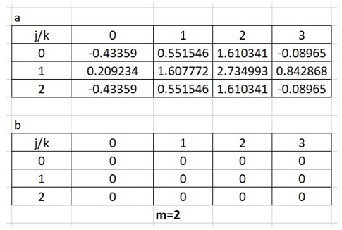
 . We compute the numbers
 ![a[4, \alpha, 0]](https://s0.wp.com/latex.php?latex=a%5B4%2C+%5Calpha%2C+0%5D&bg=ffffff&fg=111111&s=0&c=20201002) ,
, ![a[4, \alpha, 1]](https://s0.wp.com/latex.php?latex=a%5B4%2C+%5Calpha%2C+1%5D&bg=ffffff&fg=111111&s=0&c=20201002) ,
, ![a[4, \alpha, 2]](https://s0.wp.com/latex.php?latex=a%5B4%2C+%5Calpha%2C+2%5D&bg=ffffff&fg=111111&s=0&c=20201002) ,
, ![b[4, \alpha, 0]](https://s0.wp.com/latex.php?latex=b%5B4%2C+%5Calpha%2C+0%5D&bg=ffffff&fg=111111&s=0&c=20201002) ,
, ![b[4, \alpha, 1]](https://s0.wp.com/latex.php?latex=b%5B4%2C+%5Calpha%2C+1%5D&bg=ffffff&fg=111111&s=0&c=20201002) and
and ![b[4, \alpha, 2]](https://s0.wp.com/latex.php?latex=b%5B4%2C+%5Calpha%2C+2%5D&bg=ffffff&fg=111111&s=0&c=20201002) using formulas (13.48) and (13.49). We get the formulas
using formulas (13.48) and (13.49). We get the formulas![a[4, \alpha, 0] = \frac{1}{2}\big\{a[2, \alpha, 0] + \cos(\pi \cdot 0/2)a[2, \alpha + \frac{\pi}{2}, 0] - \sin(\pi \cdot 0/2)b[2, \alpha + \frac{\pi}{2}, 0]\big\}](https://s0.wp.com/latex.php?latex=a%5B4%2C+%5Calpha%2C+0%5D+%3D+%5Cfrac%7B1%7D%7B2%7D%5Cbig%5C%7Ba%5B2%2C+%5Calpha%2C+0%5D+%2B+%5Ccos%28%5Cpi+%5Ccdot+0%2F2%29a%5B2%2C+%5Calpha+%2B+%5Cfrac%7B%5Cpi%7D%7B2%7D%2C+0%5D+-+%5Csin%28%5Cpi+%5Ccdot+0%2F2%29b%5B2%2C+%5Calpha+%2B+%5Cfrac%7B%5Cpi%7D%7B2%7D%2C+0%5D%5Cbig%5C%7D&bg=ffffff&fg=111111&s=0&c=20201002)
![= \frac{1}{2}\big\{a[2, \frac{2\pi \cdot k}{8}, 0] + a[2, \frac{2\pi}{8}(k + 2), 0]\big\}](https://s0.wp.com/latex.php?latex=%3D+%5Cfrac%7B1%7D%7B2%7D%5Cbig%5C%7Ba%5B2%2C+%5Cfrac%7B2%5Cpi+%5Ccdot+k%7D%7B8%7D%2C+0%5D+%2B+a%5B2%2C+%5Cfrac%7B2%5Cpi%7D%7B8%7D%28k+%2B+2%29%2C+0%5D%5Cbig%5C%7D&bg=ffffff&fg=111111&s=0&c=20201002)
![a[4, \alpha, 1] = \frac{1}{2}\big\{a[2, \alpha, 1] + \cos(\pi \cdot 1/2)a[2, \alpha + \frac{\pi}{2}, 1] - \sin(\pi \cdot 1/2)b[2, \alpha + \frac{\pi}{2}, 1]\big\}](https://s0.wp.com/latex.php?latex=a%5B4%2C+%5Calpha%2C+1%5D+%3D+%5Cfrac%7B1%7D%7B2%7D%5Cbig%5C%7Ba%5B2%2C+%5Calpha%2C+1%5D+%2B+%5Ccos%28%5Cpi+%5Ccdot+1%2F2%29a%5B2%2C+%5Calpha+%2B+%5Cfrac%7B%5Cpi%7D%7B2%7D%2C+1%5D+-+%5Csin%28%5Cpi+%5Ccdot+1%2F2%29b%5B2%2C+%5Calpha+%2B+%5Cfrac%7B%5Cpi%7D%7B2%7D%2C+1%5D%5Cbig%5C%7D&bg=ffffff&fg=111111&s=0&c=20201002)
![= \frac{1}{2}a[2, \frac{2\pi \cdot k}{8}, 1]](https://s0.wp.com/latex.php?latex=%3D+%5Cfrac%7B1%7D%7B2%7Da%5B2%2C+%5Cfrac%7B2%5Cpi+%5Ccdot+k%7D%7B8%7D%2C+1%5D&bg=ffffff&fg=111111&s=0&c=20201002)
![a[4, \alpha, 2] = \frac{1}{2}\big\{a[2, \alpha, 2] + \cos(\pi \cdot 2/2)a[2, \alpha + \frac{\pi}{2}, 2] - \sin(\pi \cdot 2/2)b[2, \alpha + \frac{\pi}{2}, 2]\big\}](https://s0.wp.com/latex.php?latex=a%5B4%2C+%5Calpha%2C+2%5D+%3D+%5Cfrac%7B1%7D%7B2%7D%5Cbig%5C%7Ba%5B2%2C+%5Calpha%2C+2%5D+%2B+%5Ccos%28%5Cpi+%5Ccdot+2%2F2%29a%5B2%2C+%5Calpha+%2B+%5Cfrac%7B%5Cpi%7D%7B2%7D%2C+2%5D+-+%5Csin%28%5Cpi+%5Ccdot+2%2F2%29b%5B2%2C+%5Calpha+%2B+%5Cfrac%7B%5Cpi%7D%7B2%7D%2C+2%5D%5Cbig%5C%7D&bg=ffffff&fg=111111&s=0&c=20201002)
![= \frac{1}{2}\big\{a[2, \frac{2\pi \cdot k}{8}, 2] - a[2, \frac{2\pi}{8}(k + 2), 2]\big\}](https://s0.wp.com/latex.php?latex=%3D+%5Cfrac%7B1%7D%7B2%7D%5Cbig%5C%7Ba%5B2%2C+%5Cfrac%7B2%5Cpi+%5Ccdot+k%7D%7B8%7D%2C+2%5D+-+a%5B2%2C+%5Cfrac%7B2%5Cpi%7D%7B8%7D%28k+%2B+2%29%2C+2%5D%5Cbig%5C%7D&bg=ffffff&fg=111111&s=0&c=20201002)
![b[4, \alpha, 0] = \frac{1}{2}\big\{b[2, \alpha, 0] + \sin(\pi \cdot 0/2)a[2, \alpha + \frac{\pi}{2}, 0] + \cos(\pi \cdot 0/2)b[2, \alpha + \frac{\pi}{2}, 0]\big\} = 0](https://s0.wp.com/latex.php?latex=b%5B4%2C+%5Calpha%2C+0%5D+%3D+%5Cfrac%7B1%7D%7B2%7D%5Cbig%5C%7Bb%5B2%2C+%5Calpha%2C+0%5D+%2B+%5Csin%28%5Cpi+%5Ccdot+0%2F2%29a%5B2%2C+%5Calpha+%2B+%5Cfrac%7B%5Cpi%7D%7B2%7D%2C+0%5D+%2B+%5Ccos%28%5Cpi+%5Ccdot+0%2F2%29b%5B2%2C+%5Calpha+%2B+%5Cfrac%7B%5Cpi%7D%7B2%7D%2C+0%5D%5Cbig%5C%7D+%3D+0&bg=ffffff&fg=111111&s=0&c=20201002)
![b[4, \alpha, 1] = \frac{1}{2}\big\{b[2, \alpha, 1] + \sin(\pi \cdot 1/2)a[2, \alpha + \frac{\pi}{2}, 1] + \cos(\pi \cdot 1/2)b[2, \alpha + \frac{\pi}{2}, 1]\big\}](https://s0.wp.com/latex.php?latex=b%5B4%2C+%5Calpha%2C+1%5D+%3D+%5Cfrac%7B1%7D%7B2%7D%5Cbig%5C%7Bb%5B2%2C+%5Calpha%2C+1%5D+%2B+%5Csin%28%5Cpi+%5Ccdot+1%2F2%29a%5B2%2C+%5Calpha+%2B+%5Cfrac%7B%5Cpi%7D%7B2%7D%2C+1%5D+%2B+%5Ccos%28%5Cpi+%5Ccdot+1%2F2%29b%5B2%2C+%5Calpha+%2B+%5Cfrac%7B%5Cpi%7D%7B2%7D%2C+1%5D%5Cbig%5C%7D&bg=ffffff&fg=111111&s=0&c=20201002)
![= \frac{1}{2} a[2, \frac{2\pi}{8}(k+2), 1]](https://s0.wp.com/latex.php?latex=%3D+%5Cfrac%7B1%7D%7B2%7D+a%5B2%2C+%5Cfrac%7B2%5Cpi%7D%7B8%7D%28k%2B2%29%2C+1%5D&bg=ffffff&fg=111111&s=0&c=20201002)
![b[4, \alpha, 2] = \frac{1}{2}\big\{b[2, \alpha, 2] + \sin(\pi \cdot 2/2)a[2, \alpha + \frac{\pi}{2}, 2] + \cos(\pi \cdot 2/2)b[2, \alpha + \frac{\pi}{2}, 2]\big\} = 0](https://s0.wp.com/latex.php?latex=b%5B4%2C+%5Calpha%2C+2%5D+%3D+%5Cfrac%7B1%7D%7B2%7D%5Cbig%5C%7Bb%5B2%2C+%5Calpha%2C+2%5D+%2B+%5Csin%28%5Cpi+%5Ccdot+2%2F2%29a%5B2%2C+%5Calpha+%2B+%5Cfrac%7B%5Cpi%7D%7B2%7D%2C+2%5D+%2B+%5Ccos%28%5Cpi+%5Ccdot+2%2F2%29b%5B2%2C+%5Calpha+%2B+%5Cfrac%7B%5Cpi%7D%7B2%7D%2C+2%5D%5Cbig%5C%7D+%3D+0&bg=ffffff&fg=111111&s=0&c=20201002)
![a[4, \frac{2\pi \cdot 0}{8}, 0] = \frac{1}{2}\big\{a[2, \frac{2\pi \cdot 0}{8}, 0] + a[2, \frac{2\pi}{8}(0 + 2), 0]\big\}](https://s0.wp.com/latex.php?latex=a%5B4%2C+%5Cfrac%7B2%5Cpi+%5Ccdot+0%7D%7B8%7D%2C+0%5D+%3D+%5Cfrac%7B1%7D%7B2%7D%5Cbig%5C%7Ba%5B2%2C+%5Cfrac%7B2%5Cpi+%5Ccdot+0%7D%7B8%7D%2C+0%5D+%2B+a%5B2%2C+%5Cfrac%7B2%5Cpi%7D%7B8%7D%280+%2B+2%29%2C+0%5D%5Cbig%5C%7D&bg=ffffff&fg=111111&s=0&c=20201002)

![a[4, \frac{2\pi \cdot 1}{8}, 0] = \frac{1}{2}\big\{a[2, \frac{2\pi \cdot 1}{8}, 0] + a[2, \frac{2\pi}{8}(1 + 2), 0]\big\}](https://s0.wp.com/latex.php?latex=a%5B4%2C+%5Cfrac%7B2%5Cpi+%5Ccdot+1%7D%7B8%7D%2C+0%5D+%3D+%5Cfrac%7B1%7D%7B2%7D%5Cbig%5C%7Ba%5B2%2C+%5Cfrac%7B2%5Cpi+%5Ccdot+1%7D%7B8%7D%2C+0%5D+%2B+a%5B2%2C+%5Cfrac%7B2%5Cpi%7D%7B8%7D%281+%2B+2%29%2C+0%5D%5Cbig%5C%7D&bg=ffffff&fg=111111&s=0&c=20201002)

![a[4, \frac{2\pi \cdot 0}{8}, 1] = \frac{1}{2}a[2, \frac{2\pi \cdot 0}{8}, 1]](https://s0.wp.com/latex.php?latex=a%5B4%2C+%5Cfrac%7B2%5Cpi+%5Ccdot+0%7D%7B8%7D%2C+1%5D+%3D+%5Cfrac%7B1%7D%7B2%7Da%5B2%2C+%5Cfrac%7B2%5Cpi+%5Ccdot+0%7D%7B8%7D%2C+1%5D&bg=ffffff&fg=111111&s=0&c=20201002)

![a[4, \frac{2\pi \cdot 1}{8}, 1] = \frac{1}{2}a[2, \frac{2\pi \cdot 1}{8}, 1]](https://s0.wp.com/latex.php?latex=a%5B4%2C+%5Cfrac%7B2%5Cpi+%5Ccdot+1%7D%7B8%7D%2C+1%5D+%3D+%5Cfrac%7B1%7D%7B2%7Da%5B2%2C+%5Cfrac%7B2%5Cpi+%5Ccdot+1%7D%7B8%7D%2C+1%5D&bg=ffffff&fg=111111&s=0&c=20201002)

![a[4, \frac{2\pi \cdot 0}{8}, 2] = \frac{1}{2}\big\{a[2, \frac{2\pi \cdot 0}{8}, 2] - a[2, \frac{2\pi}{8}(0 + 2), 2]\big\}](https://s0.wp.com/latex.php?latex=a%5B4%2C+%5Cfrac%7B2%5Cpi+%5Ccdot+0%7D%7B8%7D%2C+2%5D+%3D+%5Cfrac%7B1%7D%7B2%7D%5Cbig%5C%7Ba%5B2%2C+%5Cfrac%7B2%5Cpi+%5Ccdot+0%7D%7B8%7D%2C+2%5D+-+a%5B2%2C+%5Cfrac%7B2%5Cpi%7D%7B8%7D%280+%2B+2%29%2C+2%5D%5Cbig%5C%7D&bg=ffffff&fg=111111&s=0&c=20201002)

![a[4, \frac{2\pi \cdot 1}{8}, 2] = \frac{1}{2}\big\{a[2, \frac{2\pi \cdot 1}{8}, 2] - a[2, \frac{2\pi}{8}(1 + 2), 2]\big\}](https://s0.wp.com/latex.php?latex=a%5B4%2C+%5Cfrac%7B2%5Cpi+%5Ccdot+1%7D%7B8%7D%2C+2%5D+%3D+%5Cfrac%7B1%7D%7B2%7D%5Cbig%5C%7Ba%5B2%2C+%5Cfrac%7B2%5Cpi+%5Ccdot+1%7D%7B8%7D%2C+2%5D+-+a%5B2%2C+%5Cfrac%7B2%5Cpi%7D%7B8%7D%281+%2B+2%29%2C+2%5D%5Cbig%5C%7D&bg=ffffff&fg=111111&s=0&c=20201002)

![b[4, \frac{2\pi \cdot 0}{8}, 0] = 0](https://s0.wp.com/latex.php?latex=b%5B4%2C+%5Cfrac%7B2%5Cpi+%5Ccdot+0%7D%7B8%7D%2C+0%5D+%3D+0&bg=ffffff&fg=111111&s=0&c=20201002)
![b[4, \frac{2\pi \cdot 1}{8}, 0] = 0](https://s0.wp.com/latex.php?latex=b%5B4%2C+%5Cfrac%7B2%5Cpi+%5Ccdot+1%7D%7B8%7D%2C+0%5D+%3D+0&bg=ffffff&fg=111111&s=0&c=20201002)
![b[4, \frac{2\pi \cdot 0}{8}, 1] = \frac{1}{2} a[2, \frac{2\pi}{8}(0+2), 1]](https://s0.wp.com/latex.php?latex=b%5B4%2C+%5Cfrac%7B2%5Cpi+%5Ccdot+0%7D%7B8%7D%2C+1%5D+%3D+%5Cfrac%7B1%7D%7B2%7D+a%5B2%2C+%5Cfrac%7B2%5Cpi%7D%7B8%7D%280%2B2%29%2C+1%5D&bg=ffffff&fg=111111&s=0&c=20201002)

![b[4, \frac{2\pi \cdot 1}{8}, 1] = \frac{1}{2} a[2, \frac{2\pi}{8}(1+2), 1]](https://s0.wp.com/latex.php?latex=b%5B4%2C+%5Cfrac%7B2%5Cpi+%5Ccdot+1%7D%7B8%7D%2C+1%5D+%3D+%5Cfrac%7B1%7D%7B2%7D+a%5B2%2C+%5Cfrac%7B2%5Cpi%7D%7B8%7D%281%2B2%29%2C+1%5D&bg=ffffff&fg=111111&s=0&c=20201002)

![b[4, \frac{2\pi \cdot 0}{8}, 2] = 0](https://s0.wp.com/latex.php?latex=b%5B4%2C+%5Cfrac%7B2%5Cpi+%5Ccdot+0%7D%7B8%7D%2C+2%5D+%3D+0&bg=ffffff&fg=111111&s=0&c=20201002)
![b[4, \frac{2\pi \cdot 1}{8}, 2] = 0](https://s0.wp.com/latex.php?latex=b%5B4%2C+%5Cfrac%7B2%5Cpi+%5Ccdot+1%7D%7B8%7D%2C+2%5D+%3D+0&bg=ffffff&fg=111111&s=0&c=20201002)
![a[4, \alpha, 3]](https://s0.wp.com/latex.php?latex=a%5B4%2C+%5Calpha%2C+3%5D&bg=ffffff&fg=111111&s=0&c=20201002) ,
, ![a[4, \alpha, 4]](https://s0.wp.com/latex.php?latex=a%5B4%2C+%5Calpha%2C+4%5D&bg=ffffff&fg=111111&s=0&c=20201002) ,
, ![b[4, \alpha, 3]](https://s0.wp.com/latex.php?latex=b%5B4%2C+%5Calpha%2C+3%5D&bg=ffffff&fg=111111&s=0&c=20201002) and
and ![b[4, \alpha, 4]](https://s0.wp.com/latex.php?latex=b%5B4%2C+%5Calpha%2C+4%5D&bg=ffffff&fg=111111&s=0&c=20201002) using equations (13.50), which tell us that
using equations (13.50), which tell us that![a[4, \alpha, 3] = a[4, \alpha, 1]](https://s0.wp.com/latex.php?latex=a%5B4%2C+%5Calpha%2C+3%5D+%3D+a%5B4%2C+%5Calpha%2C+1%5D&bg=ffffff&fg=111111&s=0&c=20201002)
![a[4, \alpha, 4] = a[4, \alpha, 0]](https://s0.wp.com/latex.php?latex=a%5B4%2C+%5Calpha%2C+4%5D+%3D+a%5B4%2C+%5Calpha%2C+0%5D&bg=ffffff&fg=111111&s=0&c=20201002)
![b[4, \alpha, 3] = -b[4, \alpha, 1]](https://s0.wp.com/latex.php?latex=b%5B4%2C+%5Calpha%2C+3%5D+%3D+-b%5B4%2C+%5Calpha%2C+1%5D&bg=ffffff&fg=111111&s=0&c=20201002)
![b[4, \alpha, 4] = -b[4, \alpha, 0]](https://s0.wp.com/latex.php?latex=b%5B4%2C+%5Calpha%2C+4%5D+%3D+-b%5B4%2C+%5Calpha%2C+0%5D&bg=ffffff&fg=111111&s=0&c=20201002)
 and
and ![a[4, \frac{2\pi \cdot 0}{8}, 3] = 0.104617](https://s0.wp.com/latex.php?latex=a%5B4%2C+%5Cfrac%7B2%5Cpi+%5Ccdot+0%7D%7B8%7D%2C+3%5D+%3D+0.104617&bg=ffffff&fg=111111&s=0&c=20201002)
![a[4, \frac{2\pi \cdot 1}{8}, 3] = 0.803886](https://s0.wp.com/latex.php?latex=a%5B4%2C+%5Cfrac%7B2%5Cpi+%5Ccdot+1%7D%7B8%7D%2C+3%5D+%3D+0.803886&bg=ffffff&fg=111111&s=0&c=20201002)
![a[4, \frac{2\pi \cdot 0}{8}, 4] = 0.5883755](https://s0.wp.com/latex.php?latex=a%5B4%2C+%5Cfrac%7B2%5Cpi+%5Ccdot+0%7D%7B8%7D%2C+4%5D+%3D+0.5883755&bg=ffffff&fg=111111&s=0&c=20201002)
![a[4, \frac{2\pi \cdot 1}{8}, 4] = 0.230946](https://s0.wp.com/latex.php?latex=a%5B4%2C+%5Cfrac%7B2%5Cpi+%5Ccdot+1%7D%7B8%7D%2C+4%5D+%3D+0.230946&bg=ffffff&fg=111111&s=0&c=20201002)
![b[4, \frac{2\pi \cdot 0}{8}, 3] = -1.3674965](https://s0.wp.com/latex.php?latex=b%5B4%2C+%5Cfrac%7B2%5Cpi+%5Ccdot+0%7D%7B8%7D%2C+3%5D+%3D+-1.3674965&bg=ffffff&fg=111111&s=0&c=20201002)
![b[4, \frac{2\pi \cdot 1}{8}, 3] = -0.421434](https://s0.wp.com/latex.php?latex=b%5B4%2C+%5Cfrac%7B2%5Cpi+%5Ccdot+1%7D%7B8%7D%2C+3%5D+%3D+-0.421434&bg=ffffff&fg=111111&s=0&c=20201002)
![b[4, \frac{2\pi \cdot 0}{8}, 4] = 0](https://s0.wp.com/latex.php?latex=b%5B4%2C+%5Cfrac%7B2%5Cpi+%5Ccdot+0%7D%7B8%7D%2C+4%5D+%3D+0&bg=ffffff&fg=111111&s=0&c=20201002)
![b[4, \frac{2\pi \cdot 1}{8}, 4] = 0](https://s0.wp.com/latex.php?latex=b%5B4%2C+%5Cfrac%7B2%5Cpi+%5Ccdot+1%7D%7B8%7D%2C+4%5D+%3D+0&bg=ffffff&fg=111111&s=0&c=20201002)
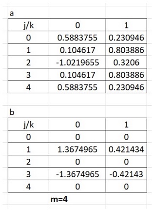
 . We compute the numbers
 ![a[8, 0, 0]](https://s0.wp.com/latex.php?latex=a%5B8%2C+0%2C+0%5D&bg=ffffff&fg=111111&s=0&c=20201002) ,
, ![a[8, 0, 1]](https://s0.wp.com/latex.php?latex=a%5B8%2C+0%2C+1%5D&bg=ffffff&fg=111111&s=0&c=20201002) ,
, ![a[8, 0, 2]](https://s0.wp.com/latex.php?latex=a%5B8%2C+0%2C+2%5D&bg=ffffff&fg=111111&s=0&c=20201002) ,
, ![a[8, 0, 3]](https://s0.wp.com/latex.php?latex=a%5B8%2C+0%2C+3%5D&bg=ffffff&fg=111111&s=0&c=20201002) ,
, ![a[8, 0, 4]](https://s0.wp.com/latex.php?latex=a%5B8%2C+0%2C+4%5D&bg=ffffff&fg=111111&s=0&c=20201002) ,
, ![b[8, 0, 0]](https://s0.wp.com/latex.php?latex=b%5B8%2C+0%2C+0%5D&bg=ffffff&fg=111111&s=0&c=20201002) ,
, ![b[8, 0, 1]](https://s0.wp.com/latex.php?latex=b%5B8%2C+0%2C+1%5D&bg=ffffff&fg=111111&s=0&c=20201002) ,
, ![b[8, 0, 2]](https://s0.wp.com/latex.php?latex=b%5B8%2C+0%2C+2%5D&bg=ffffff&fg=111111&s=0&c=20201002) ,
, ![b[8, 0, 3]](https://s0.wp.com/latex.php?latex=b%5B8%2C+0%2C+3%5D&bg=ffffff&fg=111111&s=0&c=20201002) and
and ![b[8, 0, 4]](https://s0.wp.com/latex.php?latex=b%5B8%2C+0%2C+4%5D&bg=ffffff&fg=111111&s=0&c=20201002) using formulas (13.48) and (13.49). We get
using formulas (13.48) and (13.49). We get![a[8, 0, 0] = \frac{1}{2}\big\{a[4, 0, 0] + \cos(\pi \cdot 0/4)a[4, 0 + \frac{\pi}{4}, 0] - \sin(\pi \cdot 0/4)b[4, 0 + \frac{\pi}{4}, 0]\big\}](https://s0.wp.com/latex.php?latex=a%5B8%2C+0%2C+0%5D+%3D+%5Cfrac%7B1%7D%7B2%7D%5Cbig%5C%7Ba%5B4%2C+0%2C+0%5D+%2B+%5Ccos%28%5Cpi+%5Ccdot+0%2F4%29a%5B4%2C+0+%2B+%5Cfrac%7B%5Cpi%7D%7B4%7D%2C+0%5D+-+%5Csin%28%5Cpi+%5Ccdot+0%2F4%29b%5B4%2C+0+%2B+%5Cfrac%7B%5Cpi%7D%7B4%7D%2C+0%5D%5Cbig%5C%7D&bg=ffffff&fg=111111&s=0&c=20201002)
![= \frac{1}{2}\big\{a[4, \frac{2\pi \cdot 0}{8}, 0] + a[4, \frac{2\pi}{8}(0 + 1), 0]\big\} = \frac{1}{2}(0.5883755 + 0.230946) = 0.40966075](https://s0.wp.com/latex.php?latex=%3D+%5Cfrac%7B1%7D%7B2%7D%5Cbig%5C%7Ba%5B4%2C+%5Cfrac%7B2%5Cpi+%5Ccdot+0%7D%7B8%7D%2C+0%5D+%2B+a%5B4%2C+%5Cfrac%7B2%5Cpi%7D%7B8%7D%280+%2B+1%29%2C+0%5D%5Cbig%5C%7D+%3D+%5Cfrac%7B1%7D%7B2%7D%280.5883755+%2B+0.230946%29+%3D+0.40966075&bg=ffffff&fg=111111&s=0&c=20201002)
![a[8, 0, 1] = \frac{1}{2}\big\{a[4, 0, 1] + \cos(\pi \cdot 1/4)a[4, 0 + \frac{\pi}{4}, 1] - \sin(\pi \cdot 1/4)b[4, 0 + \frac{\pi}{4}, 1]\big\}](https://s0.wp.com/latex.php?latex=a%5B8%2C+0%2C+1%5D+%3D+%5Cfrac%7B1%7D%7B2%7D%5Cbig%5C%7Ba%5B4%2C+0%2C+1%5D+%2B+%5Ccos%28%5Cpi+%5Ccdot+1%2F4%29a%5B4%2C+0+%2B+%5Cfrac%7B%5Cpi%7D%7B4%7D%2C+1%5D+-+%5Csin%28%5Cpi+%5Ccdot+1%2F4%29b%5B4%2C+0+%2B+%5Cfrac%7B%5Cpi%7D%7B4%7D%2C+1%5D%5Cbig%5C%7D&bg=ffffff&fg=111111&s=0&c=20201002)
![= \frac{1}{2}\big\{a[4, \frac{2\pi \cdot 0}{8}, 1] + \frac{1}{\sqrt{2}}a[4, \frac{2\pi}{8}(0 + 1), 1] -\frac{1}{\sqrt{2}}b[4, \frac{2\pi}{8}(0 + 1), 1]\big\}](https://s0.wp.com/latex.php?latex=%3D+%5Cfrac%7B1%7D%7B2%7D%5Cbig%5C%7Ba%5B4%2C+%5Cfrac%7B2%5Cpi+%5Ccdot+0%7D%7B8%7D%2C+1%5D+%2B+%5Cfrac%7B1%7D%7B%5Csqrt%7B2%7D%7Da%5B4%2C+%5Cfrac%7B2%5Cpi%7D%7B8%7D%280+%2B+1%29%2C+1%5D+-%5Cfrac%7B1%7D%7B%5Csqrt%7B2%7D%7Db%5B4%2C+%5Cfrac%7B2%5Cpi%7D%7B8%7D%280+%2B+1%29%2C+1%5D%5Cbig%5C%7D&bg=ffffff&fg=111111&s=0&c=20201002)

![a[8, 0, 2] = \frac{1}{2}\big\{a[4, 0, 2] + \cos(\pi \cdot 2/4)a[4, 0 + \frac{\pi}{4}, 2] - \sin(\pi \cdot 2/4)b[4, 0 + \frac{\pi}{4}, 2]\big\}](https://s0.wp.com/latex.php?latex=a%5B8%2C+0%2C+2%5D+%3D+%5Cfrac%7B1%7D%7B2%7D%5Cbig%5C%7Ba%5B4%2C+0%2C+2%5D+%2B+%5Ccos%28%5Cpi+%5Ccdot+2%2F4%29a%5B4%2C+0+%2B+%5Cfrac%7B%5Cpi%7D%7B4%7D%2C+2%5D+-+%5Csin%28%5Cpi+%5Ccdot+2%2F4%29b%5B4%2C+0+%2B+%5Cfrac%7B%5Cpi%7D%7B4%7D%2C+2%5D%5Cbig%5C%7D&bg=ffffff&fg=111111&s=0&c=20201002)
![= \frac{1}{2}a[4, \frac{2\pi \cdot 0}{8}, 2] = \frac{1}{2} \cdot (-1.0219655) = -0.51098275](https://s0.wp.com/latex.php?latex=%3D+%5Cfrac%7B1%7D%7B2%7Da%5B4%2C+%5Cfrac%7B2%5Cpi+%5Ccdot+0%7D%7B8%7D%2C+2%5D+%3D+%5Cfrac%7B1%7D%7B2%7D+%5Ccdot+%28-1.0219655%29+%3D+-0.51098275&bg=ffffff&fg=111111&s=0&c=20201002)
![a[8, 0, 3] = \frac{1}{2}\big\{a[4, 0, 3] + \cos(\pi \cdot 3/4)a[4, 0 + \frac{\pi}{4}, 3] - \sin(\pi \cdot 3/4)b[4, 0 + \frac{\pi}{4}, 3]\big\}](https://s0.wp.com/latex.php?latex=a%5B8%2C+0%2C+3%5D+%3D+%5Cfrac%7B1%7D%7B2%7D%5Cbig%5C%7Ba%5B4%2C+0%2C+3%5D+%2B+%5Ccos%28%5Cpi+%5Ccdot+3%2F4%29a%5B4%2C+0+%2B+%5Cfrac%7B%5Cpi%7D%7B4%7D%2C+3%5D+-+%5Csin%28%5Cpi+%5Ccdot+3%2F4%29b%5B4%2C+0+%2B+%5Cfrac%7B%5Cpi%7D%7B4%7D%2C+3%5D%5Cbig%5C%7D&bg=ffffff&fg=111111&s=0&c=20201002)
![= \frac{1}{2}\big\{a[4, \frac{2\pi \cdot 0}{8}, 3] - \frac{1}{\sqrt{2}}a[4, \frac{2\pi}{8}(0 + 1), 3] -\frac{1}{\sqrt{2}}b[4, \frac{2\pi}{8}(0 + 1), 3]\big\}](https://s0.wp.com/latex.php?latex=%3D+%5Cfrac%7B1%7D%7B2%7D%5Cbig%5C%7Ba%5B4%2C+%5Cfrac%7B2%5Cpi+%5Ccdot+0%7D%7B8%7D%2C+3%5D+-+%5Cfrac%7B1%7D%7B%5Csqrt%7B2%7D%7Da%5B4%2C+%5Cfrac%7B2%5Cpi%7D%7B8%7D%280+%2B+1%29%2C+3%5D+-%5Cfrac%7B1%7D%7B%5Csqrt%7B2%7D%7Db%5B4%2C+%5Cfrac%7B2%5Cpi%7D%7B8%7D%280+%2B+1%29%2C+3%5D%5Cbig%5C%7D&bg=ffffff&fg=111111&s=0&c=20201002)

![a[8, 0, 4] = \frac{1}{2}\big\{a[4, 0, 4] + \cos(\pi \cdot 4/4)a[4, 0 + \frac{\pi}{4}, 4] - \sin(\pi \cdot 4/4)b[4, 0 + \frac{\pi}{4}, 4]\big\}](https://s0.wp.com/latex.php?latex=a%5B8%2C+0%2C+4%5D+%3D+%5Cfrac%7B1%7D%7B2%7D%5Cbig%5C%7Ba%5B4%2C+0%2C+4%5D+%2B+%5Ccos%28%5Cpi+%5Ccdot+4%2F4%29a%5B4%2C+0+%2B+%5Cfrac%7B%5Cpi%7D%7B4%7D%2C+4%5D+-+%5Csin%28%5Cpi+%5Ccdot+4%2F4%29b%5B4%2C+0+%2B+%5Cfrac%7B%5Cpi%7D%7B4%7D%2C+4%5D%5Cbig%5C%7D&bg=ffffff&fg=111111&s=0&c=20201002)
![= \frac{1}{2}(a[4, \frac{2\pi \cdot 0}{8}, 4] - a[4, \frac{2\pi}{8}(0 + 1), 4]) = \frac{1}{2} (0.5883755 - 0.230946) = 0.17871475](https://s0.wp.com/latex.php?latex=%3D+%5Cfrac%7B1%7D%7B2%7D%28a%5B4%2C+%5Cfrac%7B2%5Cpi+%5Ccdot+0%7D%7B8%7D%2C+4%5D+-+a%5B4%2C+%5Cfrac%7B2%5Cpi%7D%7B8%7D%280+%2B+1%29%2C+4%5D%29+%3D+%5Cfrac%7B1%7D%7B2%7D+%280.5883755+-+0.230946%29+%3D+0.17871475&bg=ffffff&fg=111111&s=0&c=20201002)
![b[8, 0, 0] = \frac{1}{2}\big\{b[4, 0, 0] + \sin(\pi \cdot 0/4)a[4, 0 + \frac{\pi}{4}, 0] + \cos(\pi \cdot 0/4)b[4, \frac{2\pi}{8}(0 + 1), 0]\big\}](https://s0.wp.com/latex.php?latex=b%5B8%2C+0%2C+0%5D+%3D+%5Cfrac%7B1%7D%7B2%7D%5Cbig%5C%7Bb%5B4%2C+0%2C+0%5D+%2B+%5Csin%28%5Cpi+%5Ccdot+0%2F4%29a%5B4%2C+0+%2B+%5Cfrac%7B%5Cpi%7D%7B4%7D%2C+0%5D+%2B+%5Ccos%28%5Cpi+%5Ccdot+0%2F4%29b%5B4%2C+%5Cfrac%7B2%5Cpi%7D%7B8%7D%280+%2B+1%29%2C+0%5D%5Cbig%5C%7D&bg=ffffff&fg=111111&s=0&c=20201002)

![b[8, 0, 1] = \frac{1}{2}\big\{b[4, 0, 1] + \sin(\pi \cdot 1/4)a[4, 0 + \frac{\pi}{4}, 1] + \cos(\pi \cdot 1/4)b[4, 0 + \frac{\pi}{4}, 1]\big\}](https://s0.wp.com/latex.php?latex=b%5B8%2C+0%2C+1%5D+%3D+%5Cfrac%7B1%7D%7B2%7D%5Cbig%5C%7Bb%5B4%2C+0%2C+1%5D+%2B+%5Csin%28%5Cpi+%5Ccdot+1%2F4%29a%5B4%2C+0+%2B+%5Cfrac%7B%5Cpi%7D%7B4%7D%2C+1%5D+%2B+%5Ccos%28%5Cpi+%5Ccdot+1%2F4%29b%5B4%2C+0+%2B+%5Cfrac%7B%5Cpi%7D%7B4%7D%2C+1%5D%5Cbig%5C%7D&bg=ffffff&fg=111111&s=0&c=20201002)
![= \frac{1}{2}(b[4, 0, 1] + \frac{1}{\sqrt{2}} \cdot a[4, \frac{2\pi}{8}(0 + 1), 1] + \frac{1}{\sqrt{2}} \cdot b[4, \frac{2\pi}{8}(0 + 1), 1])](https://s0.wp.com/latex.php?latex=%3D+%5Cfrac%7B1%7D%7B2%7D%28b%5B4%2C+0%2C+1%5D+%2B+%5Cfrac%7B1%7D%7B%5Csqrt%7B2%7D%7D+%5Ccdot+a%5B4%2C+%5Cfrac%7B2%5Cpi%7D%7B8%7D%280+%2B+1%29%2C+1%5D+%2B+%5Cfrac%7B1%7D%7B%5Csqrt%7B2%7D%7D+%5Ccdot+b%5B4%2C+%5Cfrac%7B2%5Cpi%7D%7B8%7D%280+%2B+1%29%2C+1%5D%29&bg=ffffff&fg=111111&s=0&c=20201002)

![b[8, 0, 2] = \frac{1}{2}\big\{b[4, 0, 2] + \sin(\pi \cdot 2/4)a[4, 0 + \frac{\pi}{4}, 2] + \cos(\pi \cdot 2/4)b[4, 0 + \frac{\pi}{4}, 2]\big\}](https://s0.wp.com/latex.php?latex=b%5B8%2C+0%2C+2%5D+%3D+%5Cfrac%7B1%7D%7B2%7D%5Cbig%5C%7Bb%5B4%2C+0%2C+2%5D+%2B+%5Csin%28%5Cpi+%5Ccdot+2%2F4%29a%5B4%2C+0+%2B+%5Cfrac%7B%5Cpi%7D%7B4%7D%2C+2%5D+%2B+%5Ccos%28%5Cpi+%5Ccdot+2%2F4%29b%5B4%2C+0+%2B+%5Cfrac%7B%5Cpi%7D%7B4%7D%2C+2%5D%5Cbig%5C%7D&bg=ffffff&fg=111111&s=0&c=20201002)
![= \frac{1}{2} \cdot a[4, \frac{2\pi}{8}(0 + 1), 2] = \frac{1}{2} \cdot 0.3206 = 0.1603](https://s0.wp.com/latex.php?latex=%3D+%5Cfrac%7B1%7D%7B2%7D+%5Ccdot+a%5B4%2C+%5Cfrac%7B2%5Cpi%7D%7B8%7D%280+%2B+1%29%2C+2%5D+%3D+%5Cfrac%7B1%7D%7B2%7D+%5Ccdot+0.3206+%3D+0.1603&bg=ffffff&fg=111111&s=0&c=20201002)
![b[8, 0, 3] = \frac{1}{2}\big\{b[4, 0, 3] + \sin(\pi \cdot 3/4)a[4, 0 + \frac{\pi}{4}, 3] + \cos(\pi \cdot 3/4)b[4, 0 + \frac{\pi}{4}, 3]\big\}](https://s0.wp.com/latex.php?latex=b%5B8%2C+0%2C+3%5D+%3D+%5Cfrac%7B1%7D%7B2%7D%5Cbig%5C%7Bb%5B4%2C+0%2C+3%5D+%2B+%5Csin%28%5Cpi+%5Ccdot+3%2F4%29a%5B4%2C+0+%2B+%5Cfrac%7B%5Cpi%7D%7B4%7D%2C+3%5D+%2B+%5Ccos%28%5Cpi+%5Ccdot+3%2F4%29b%5B4%2C+0+%2B+%5Cfrac%7B%5Cpi%7D%7B4%7D%2C+3%5D%5Cbig%5C%7D&bg=ffffff&fg=111111&s=0&c=20201002)
![= \frac{1}{2}(b[4, 0, 3] + \frac{1}{\sqrt{2}} \cdot a[4, \frac{2\pi}{8}(0 + 1), 3] - \frac{1}{\sqrt{2}} \cdot b[4, \frac{2\pi}{8}(0 + 1), 3])](https://s0.wp.com/latex.php?latex=%3D+%5Cfrac%7B1%7D%7B2%7D%28b%5B4%2C+0%2C+3%5D+%2B+%5Cfrac%7B1%7D%7B%5Csqrt%7B2%7D%7D+%5Ccdot+a%5B4%2C+%5Cfrac%7B2%5Cpi%7D%7B8%7D%280+%2B+1%29%2C+3%5D+-+%5Cfrac%7B1%7D%7B%5Csqrt%7B2%7D%7D+%5Ccdot+b%5B4%2C+%5Cfrac%7B2%5Cpi%7D%7B8%7D%280+%2B+1%29%2C+3%5D%29&bg=ffffff&fg=111111&s=0&c=20201002)

![b[8, 0, 4] = \frac{1}{2}\big\{b[4, 0, 4] + \sin(\pi \cdot 4/4)a[4, 0 + \frac{\pi}{4}, 4] + \cos(\pi \cdot 4/4)b[4, 0 + \frac{\pi}{4}, 4]\big\} = 0](https://s0.wp.com/latex.php?latex=b%5B8%2C+0%2C+4%5D+%3D+%5Cfrac%7B1%7D%7B2%7D%5Cbig%5C%7Bb%5B4%2C+0%2C+4%5D+%2B+%5Csin%28%5Cpi+%5Ccdot+4%2F4%29a%5B4%2C+0+%2B+%5Cfrac%7B%5Cpi%7D%7B4%7D%2C+4%5D+%2B+%5Ccos%28%5Cpi+%5Ccdot+4%2F4%29b%5B4%2C+0+%2B+%5Cfrac%7B%5Cpi%7D%7B4%7D%2C+4%5D%5Cbig%5C%7D+%3D+0&bg=ffffff&fg=111111&s=0&c=20201002)


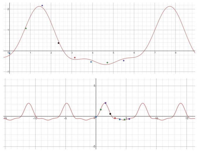

![[0.01, 0.06]](https://s0.wp.com/latex.php?latex=%5B0.01%2C+0.06%5D&bg=ffffff&fg=111111&s=0&c=20201002) . I plotted this in Python as follows:
. I plotted this in Python as follows: 

 denote an
  data matrix, e.g., observations on
  denotes the transpose of
  matrix
  is
is  -times the covariance matrix of the data. Since
  for
for  , and corresponding orthonormal eingenvectors
  ,
,  , and we can then write the eigenvalue equations in matrix form as
 is a
is a  is a
is a  of the data set onto its principal directions. The
  is thus used for data dimensionality reduction. The idea is that the first two or three columns of the

 is the covariance matrix of
  instead of
  . To clarify this, note that
 ![\text{tr}[(\mathbf{X} \mathbf{V})' (\mathbf{X} \mathbf{V})] = \text{tr}(\mathbf{V}' \mathbf{X}'\mathbf{X}\mathbf{V}) = \text{tr}(\mathbf{X}'\mathbf{X}\mathbf{V}\mathbf{V}') \leq \sum_{i=1}^k \lambda_i(\mathbf{X}'\mathbf{X}) \lambda_i(\mathbf{V}\mathbf{V}')](https://s0.wp.com/latex.php?latex=%5Ctext%7Btr%7D%5B%28%5Cmathbf%7BX%7D+%5Cmathbf%7BV%7D%29%27+%28%5Cmathbf%7BX%7D+%5Cmathbf%7BV%7D%29%5D+%3D+%5Ctext%7Btr%7D%28%5Cmathbf%7BV%7D%27+%5Cmathbf%7BX%7D%27%5Cmathbf%7BX%7D%5Cmathbf%7BV%7D%29+%3D+%5Ctext%7Btr%7D%28%5Cmathbf%7BX%7D%27%5Cmathbf%7BX%7D%5Cmathbf%7BV%7D%5Cmathbf%7BV%7D%27%29+%5Cleq+%5Csum_%7Bi%3D1%7D%5Ek+%5Clambda_i%28%5Cmathbf%7BX%7D%27%5Cmathbf%7BX%7D%29+%5Clambda_i%28%5Cmathbf%7BV%7D%5Cmathbf%7BV%7D%27%29&bg=ffffff&fg=111111&s=0&c=20201002)
 ,
,  , represents the eigenvalues of a matrix
  , so that
  and
and ![\text{tr}[(\mathbf{X} \mathbf{V})' (\mathbf{X} \mathbf{V})] = \sum_{i=1}^k \lambda_i(\mathbf{X}'\mathbf{X})](https://s0.wp.com/latex.php?latex=%5Ctext%7Btr%7D%5B%28%5Cmathbf%7BX%7D+%5Cmathbf%7BV%7D%29%27+%28%5Cmathbf%7BX%7D+%5Cmathbf%7BV%7D%29%5D+%3D+%5Csum_%7Bi%3D1%7D%5Ek+%5Clambda_i%28%5Cmathbf%7BX%7D%27%5Cmathbf%7BX%7D%29&bg=ffffff&fg=111111&s=0&c=20201002)

 is an orthogonal
  matrix containing the eigenvectors of the
  ,
,  is an
is an 