A mathematics and physics `scrapbook', with notes on miscellaneous things that catch my interest in a range of areas including: mathematical methods; number theory; probability theory; stochastic processes; mathematical economics; econometrics; quantum theory; relativity theory; cosmology; cloud physics; statistical mechanics; nonlinear dynamics; electronic engineering; graph and network theory; mathematics in Latin; computational mathematics using Python and other maths software.
The Legendre transform is a mechanism for converting a relationship like
into a relationship like
In other words, by going from a function to its Legendre transform and vice versa, the roles of and in (1) and (2) can be reversed.
In moving from (1) to (2), the required Legendre transform is
because differentiating both sides of (3) with respect to gives
Using (1), we see that the last two terms in (4) cancel, so we get (2). Conversely, the Legendre transform of in (2) can be written
because differentiating both sides with respect to gives (1).
Mainly for teaching purposes, I want to consider a simple example here of applying the Legendre transform to the conversion of a Lagrangian mechanics problem into an equivalent Hamiltonian one. We might want to do this for a number of reasons, not least because it converts the problem of solving second-order ODEs in the case of the Lagrangian formulation into a potentially simpler problem of solving first-order ODEs in the case of the Hamiltonian formulation.
Consider a simple harmonic oscillator consisting of a mass attached to a spring with spring constant moving backwards and forwards horizontally on a frictionless table. There is a restoring force that wants to bring the mass back towards its equilibrium position whenever it is displaced either by compressing the spring or stretching it. Newton’s second law, , then gives us the second-order ODE
with general solution
where is the natural frequency of this system’s oscillations. We could obtain a particular solution (i.e., provide specific values for and ) given a pair of initial conditions, e.g., the initial conditions and would give us the particular solution
The dynamics of this system are now completely determined and we can specify the values of , and at any point in time .
As is well known, we can arrive at exactly the same result using Lagrangian mechanics, which involves writing the Lagrangian for the problem as
where is kinetic energy and is potential energy. For the simple harmonic oscillator we have
and
Therefore, the Lagrangian for the harmonic oscillator problem is
We define the action as the functional
and seek the extremal function at which the action is stationary. The extremal is obtained by solving for the first-order condition for this optimisation problem, known as the Euler-Lagrange equation:
Applying the Euler-Lagrange equation to the Lagrangian for the harmonic oscillator problem in (12) we find
which is the same as the ODE in (6) obtained by Newtonian mechanics.
[To briefly explain how the Euler-Lagrange equation is derived, we begin by constructing a function , where is the desired extremal, is a parameter, and denotes a function which goes through the same two endpoints and as the extremal, but has zero value at these endpoints. The new function then represents the set of all possible varied curves that can joint the two endpoints. Out of all of these curves, we want the one that makes the action stationary, where the action is now treated as the function of given by . That is, we want when . Noting that and and differentiating under the integral sign we get
Setting and at this point, which is what is required, and remembering that means , we obtain
To convert the second term in this integrand into something multiplying instead of , we can use integration by parts to get
Putting this result into the previous integral we get
from which the Euler-Lagrange equation in (14) follows since is arbitrary.]
We now want to see how this can be transformed into a Hamiltonian mechanics problem using the Legendre transform outlined earlier. We begin by defining a new variable to replace the partial , which is usually referred to as the generalised momentum in the mechanics literature:
(In the case of the simple harmonic oscillator problem, this will turn out to be the actual linear momentum. The other partial in the Euler-Lagrange equation, , is usually referred to as the generalised force in the mechanics literature, and again will turn out to be the actual force in the case of the simple harmonic oscillator). We now regard (15) as the analogue of equation (1). It follows that the analogue of equation (2) must then be
where is the Legendre transform that takes us from (15) to (16), namely
This is the analogue of (3). This Legendre transform now enables us to write down the Hamiltonian for the harmonic oscillator problem, starting from the Lagrangian in (12). We begin by using (15) to obtain
which allows us to replace by wherever it occurs. Then using (12) in (17) with instead of we get
Therefore, we see that whereas , the Legendre transform has instead given us . We can also get an equation in terms of for the Euler-Lagrange equation in (14) above by noting from (17) that
and from (18) that
Therefore, the Euler-Lagrange condition for making the action stationary can be written in terms of as the pair of equations
which is just (16) and represents the act of carrying out the Legendre transform, and
which from (20) and (21) represents the Euler-Lagrange condition expressed in terms of the Hamiltonian. These two first-order ODEs are usually referred to as Hamilton’s equations, and are often more convenient to solve than the second-order ODEs arising in Lagrangian mechanics. The fact that the Hamiltonian is expressed in terms and and represents the total energy of the system also allows geometric insights to be conveniently obtained, e.g., by plotting constant-energy contours for the system in a x-p phase space. All of this means that, when faced with a mechanics problem, we can usually simply state the Hamiltonian as , then use Hamilton’s equations as the first-order conditions for making the action stationary, as long as we know the kinetic energy and the potential energy for the problem in terms of and .
In the case of the simple harmonic oscillator, Hamilton’s equations give us
and
From (22) we get
and equating this with (23) we get
which again is the same as the ODE in (6) obtained from Newtonian mechanics.
Finally, it is obvious from the form of the Hamiltonian in (19) that the level sets of for the simple harmonic oscillator, i.e., the constant-energy contours in x-p phase space, will be circular orbits as shown in the diagram.
A heat flow problem led to the following general series solution:
An initial condition at required , so it was necessary to find the coefficients in the following sine series:
The sine functions here involve coefficients of of the form rather than the usual . They have period and by looking at graphs it is easy to convince oneself that
so
Also, orthogonality can be demonstrated in the usual ways (e.g., using the exponential form of the sine function):
for . In fact, the functions for form a complete, orthogonal set of basis functions and we can expand in this basis. To this end, we need to create an odd function involving of the form
The coefficients of the Fourier sine series are then obtained as
The full solution of the heat flow problem is thus
Bessel’s equation arises in countless physics applications and has the form
where the constant is known as the order of the Bessel function which solves (1). The method of Frobenius can be used to find series solutions for of the form
where is a number to be found by substituting (2) and its relevant derivatives into (1). We assume that is not zero, so the first term of the series will be . Successive differentiation of (2) and substitution into (1) produces for each power of in (2) an equation equal to zero involving combinations of several coefficients . (The total coefficient of each power of must be zero to ensure the right-hand side of (1) ends up as zero). The equation for the coefficient of is used to find the possible values of and is known as the indicial equation. For the Bessel equation in (1), this procedure results in the indicial equation
so and we need to find two solutions, one for and another for . A linear combination of these two solutions can then be used to construct a general solution of (1). The Frobenius procedure also leads to = 0 and the following recursion formula for the remaining coefficients:
We use this to find coefficients for first, and can then simply replace by to get the coefficients for . Here, we focus only on the case which upon substitution in (3) gives
Evaluating these coefficients with a starting value of results in solutions called Bessel functions of the first kind and order , usually denoted by . In the present note, I am concerned only with the Bessel function of the first kind and order zero, , obtained by setting . We then have a starting value and we obtain the following coefficients in the power series for :
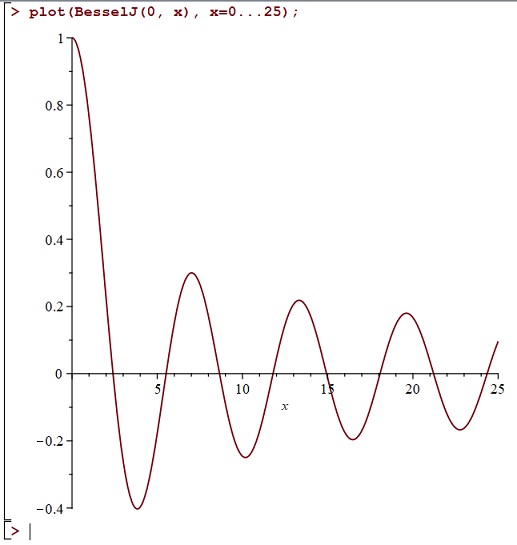
and so on. So, leads to all odd-numbered coefficients being zero and we end up with the following generalized series expression for the Bessel function of the first kind and order zero:
We can easily plot using MAPLE and it looks like a kind of damped cosine function. Here is a quick plot for positive values of :
The series in (5) above is given, albeit in a more general complex variable setting, as equation (3) on page 16 in the classic work by G. N. Watson, 1922, A Treatise On The Theory of Bessel Functions, Cambridge University Press. (At the time of writing, this monumental book is freely downloadable from several online sites). In the present note, I am interested in certain integral formulae which give rise to the same series as (5). These are discussed in Chapter Two of Watson’s treatise, and I want to unpick some things from there. In particular, I am intrigued by the following passage on pages 19 and 20 of Watson’s book:
In the remainder of this note, I want to obtain the series for in (5) above directly from the integral in equation (1) in this extract from Watson’s book, adapted to the real-variable case with . I also want to use Watson’s technique of bisecting the range of integration to obtain a clear intuitive understanding of other equivalent integral formulae for .
Begin by setting and in the integral in (1) in the extract to get
To confirm the validity of this, we can substitute into the Taylor series expansion for , namely
to get
Now integrate both sides of (7) from to , using a formula I explored in a previous note for integrating even powers of the sine function, namely
We obtain
so
Thus, (6) holds. Notice that the integral in (6) is the average value of the integrand over the interval from to . Looking at graphs of the sine and cosine functions, we can easily imagine that we can switch between the two and that this average also remains unchanged if we restrict the range of integration to the interval from to , and divide the integral by instead of .
Thus, it seems intuitively obvious that the following are equivalent integral formulae for :
In addition, if we substitute into the Taylor series expansion for , namely
we get
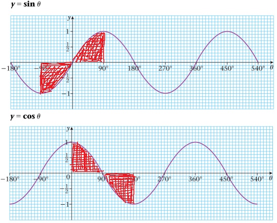
But when we integrate both sides of this from to , the odd terms on the right-hand side will vanish and the even terms will be the same as they were in the derivation of (9) above using the Taylor series for cos. We thus obtain another equivalent integral formula for :
Furthermore, we can again restrict the range of integration in (12) and switch between sine and cosine as indicated in the following graphs:
Thus, we obtain the following equivalent integral formulae for :
We can imagine easily obtaining many other equivalent integral formulae for in this way.
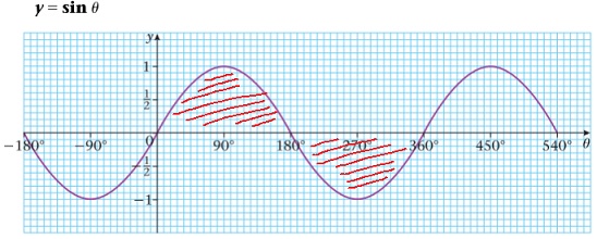
I needed to integrate increasing odd and even integer powers of the sine function repeatedly in a power series, with limits from to . Looking at the graph of the sine function, it is obvious that since sine is itself an odd function its odd powers must integrate to zero over the interval from to (intuitively, negatively signed areas will cancel positively signed ones).
For the even integer powers, I found the following definite integral formula with limits to in the standard reference book by I. S. Gradshteyn and I. M. Ryzhik, 1994, Table of Integrals, Series and Products, page 412:
The double exclamation marks mean that we deduct 2 to get each subsequent term in the factorial, so
and
.
The symmetry of the graph and the fact that even powers of sine are even functions suggest that the right-hand side of (1) only needs to be multiplied by 4 to get the correct definite integral formula for the interval to . Thus, we obtain the following useful formula for integrating integer powers of sine over a full period:
For peace of mind, I also wanted to prove the formula in (2) by direct integration and I found a way of doing this using integration by parts as follows. We have
Therefore,
so
Continuing this pattern recursively with the integral on the right-hand side we get
From the pattern of the numerators we see that this evaluates to zero if is odd and to
A basic result from applying Gauss’ Law of electromagnetism to a conductor is that any excess charge always ends up distributed entirely on the surface of the conductor. Furthermore, the excess charge will always distribute itself there so as to produce an equipotential surface. The resulting surface charge density distribution per unit area is usually difficult to obtain as a formula in closed form but it happens to be known for a conducting ellipsoid with general equation
If the total excess charge on the surface of this conducting ellipsoid is , the distribution of surface charge density per unit area is given by
(see, e.g., D. Griffiths, 1999, Introduction to Electrodynamics, Problem 2.52, page 109). Interestingly, it is possible to deduce from this the surface charge density distribution of other conducting solids that can be obtained as special cases of a conducting ellipsoid by suitable choices for the parameters , and , and I wanted to make a note of this here.
For example, we can immediately obtain the surface charge density distribution of a conducting sphere of radius by setting in (1) and (2) above to get the sphere
and its corresponding surface charge density
where the last equality follows by (3).
Note that a unit sphere
can be transformed into the ellipsoid in (1) above via a scaling of each of the variables, i.e., the change of variables , , . Thus, we can obtain the surface charge density of a circular conducting disk of radius coplanar with the -plane and with centre at the origin by setting and in (2), and using the fact that on the surface of the ellipsoid we have
so that (2) can be rearranged to read
Thus, setting and in (7), we get the following formula for the surface charge density per unit area of a circular conducting disk of radius and total excess charge (spread over both sides) at a point a radial distance from its centre:
I recently needed to integrate the fifth power of a sine function from zero to and did this via a hypergeometric function, which I found quite interesting. I will make a quick note of it here. I came across the following entry in a table of integrals:
The function is a special function known as the ordinary hypergeometric function. The required definite integral for , and limits to is then
What interested me is that there is a summation theorem for the case which yields a simple ratio of products of the gamma function when :
Since this condition happens to be satisfied in our case, we thus have
When confronted with a first-order differential equation, try to convert it to one of these five basic types:
1). Separable: This is when can be written . If there is an initial condition , we can rearrange to get an equation involving two integrals:
This incorporates the initial condition. It can sometimes be solved to give a solution in the form . Note the following integration tricks which are sometimes useful here:
2). Homogeneous: These equations are those for which depends only the ratio rather than on and separately. So, they are of the form with initial condition . To transform this into a separable equation, make the change of variable . Then , so we have and therefore . The initial condition becomes , so . The method of separation of variables can now be applied to the transformed equation.
3). Non-separable linear first-order equations: These have the general form , with boundary condition . Here, we need to find an integrating factor that allows us to write the differential equation as
Expanding this form, we find that
and so
This shows that in the original equation we must have and therefore the required integrating factor is . So what we do is find the integrating factor, then write the equation in the form . This can then be solved by integration to get where is a constant of integration. If the integral constant cannot be evaluated directly, it is best to give the solution as
because this expression automatically satisfies the boundary condition (when , the integral vanishes and so the equation reduces to ).
4). Bernoulli’s equation: This is a nonlinear first-order equation of the form . To solve this, make the change of variable . Then , so the original equation can be rewritten as
This is now a linear first-order equation of the type 3) above.
5). Riccati’s equation: This is a nonlinear first-order equation of the form . It reduces to a linear equation if and Bernoulli’s equation if . Otherwise, it can be reduced to a linear second-order equation by defining a new dependent variable with the equation . This converts the original Riccati equation into
which can be solved using known methods depending on the specific details of each case.
My first academic job was as a lecturer in economics at Royal Holloway, University of London, where I was responsible for the second-year mathematical methods and econometrics course EC2203 Quantitative Methods in Economics II. I have lost all the original manuscripts of the lecture notes but still have scanned copies of most of the printouts (only Lecture 18 Estimation of structural equations is lost forever, unfortunately!) I am posting them here in the order in which I delivered them.
The present note uses the setup outlined in a previous note about a 2016 paper in Physical Review Letters on the large deviation analysis of rapid-onset rain showers. This paper will be referred to as MW2016 herein. In order to apply large deviation theory to a collector-drop framework for rapid-onset rain formation, equation [14] in MW2016 presents the cumulant generating function for the random variable , which I will write here as
The Laplace transform of the required probability density is , so equation [15] in MW2016 sets up a relevant Bromwich integral equation, which I will write here as
At first sight, this seems intractable directly, and a saddle-point approximation for the density in (1) is presented in equation [17] in MW2016. This saddle-point approximation involves the large deviation entropy function for the random variable , and an intricate asymptotic analysis is then embarked upon to obtain an explicit expression for this entropy function. The result is the expression given in equation [24] in MW2016.
However, instead of approximating (1), it is possible to work out the Bromwich integral exactly. The result is the exact version of the probability density which is approximated in equation [17] in MW2016. This is a known distribution called the generalised Erlang distribution, but I have not been able to find any derivations of it using the Bromwich integral approach. Typically, derivations are carried out using characteristic functions (see, e.g., Bibinger, M., 2013, Notes on the sum and maximum of independent exponentially distributed random variables with different scale parameters, arXiv:1307.3945 [math.PR]), or phase-type distribution methods (see, e.g., O’Cinneide, C., 1999, Phase-type distribution: open problems and a few properties, Communication in Statistic-Stochastic Models, 15(4), pp. 731-757).
To derive this distribution directly from the Bromwich integral in (1), begin by replacing the term by the product it gives rise to:
Then, starting from an elementary bivariate partial fraction expansion, and extending this to variables by induction, we can obtain the following expression for the product term in (2):
The detailed derivation of (3) is set out in an Appendix below. Putting (3) back into (2), and moving the integral sign `through’ the summation and product in (3), we obtain the following form for the Bromwich integral:
Each integrand in (4) has a simple pole at , so the residue at each such singularity is given by
We can construct a contour in the complex plane which is appropriate for each by creating a semicircle with the straight vertical part located at a point to the right of , and with the arc of the semicircle large enough to enclose the point on the real axis (diagram below). Since is the smallest collision rate, and is the largest, this ensures that the contour will enclose each point.
It then follows by Cauchy’s residue theorem, and the fact that the integral along the circular arc component of the contour vanishes as the radius of the semicircle goes to infinity, that
Putting (6) in (4), we then get the exact form of the required density:
This is the density function of the generalised Erlang distribution, and is given in an alternative (but equivalent) form in equation [SB1.1] on page 241 of a paper by Kostinski and Shaw (Kostinski, A., Shaw, R., 2005, Fluctuations and Luck in Droplet Growth by Coalescence, Bull. Am. Meteorol. Soc. 86, 235). Integrating (7) with respect to , we obtain the cumulative distribution function
Again this is given in an alternative (but equivalent) form on page 241 of Kostinski and Shaw’s paper, as equation [SB1.2].
Although we now have the exact pdf and cdf corresponding to the Bromwich integral in MW2016, these are not practical for calculations in the context of runaway raindrop growth. This runaway process can involve large numbers of water particle collisions , e.g., , so the expressions in (7) and (8) would involve sums of thousands of product terms, each of these products in turn involving thousands of terms. Therefore, we are still interested in obtaining a formula for the entropy function to enable large deviation approximations for (7) and (8) for practical calculations. It may be possible to obtain an approximation for the entropy function directly from the cdf in (8), but this would require further investigation.
An initial problem that might need to be overcome is that the forms for the cdf in (8) above and also in Kostinski and Shaw (which is similar) are inconvenient. However, they can be manipulated as follows. First, expand (8) to obtain
A recent paper by Yanev (Yanev, G., 2020, Exponential and Hypoexponential Distributions: Some Characterizations, Mathematics, 8(12), 2207) pointed out that the product terms appearing in (9) are related to the terms appearing in the Lagrange polynomial interpolation formula. This formula and its properties are well known in the field of approximation theory (see, e.g., pages 33-35 in Powell, M., 1981, Approximation Theory and Methods, Cambridge University Press). This fact was used in a paper by Sen and Balakrishnan (Sen, A., Balakrishnan, N., 1999, Convolution of geometrics and a reliability problem, Statistics & Probability Letters, 43, pp. 421-426) to give a simple proof that the sum/product which appears as the first term on the right-hand side of (9) is identically equal to 1:
(See my previous note about this). Using (10) in (9), we then obtain the cdf in a potentially more convenient form:
Appendix: Proof of the partial fraction expansion in (3)
The following arguments use the Lagrange polynomial interpolation formula to prove the partial fraction expansion in (3) above. We will need formula (6) in my previous note about this, which is repeated here for convenience:
To prove (3) above, we begin by using Lagrange’s polynomial interpolation formula to prove the following auxiliary result:
Taking apart (12) above (which equals 1) and using (10) above, we obtain
Therefore we conclude
We will need this result shortly. Next, we expand the bracketed terms on the left-hand side of (13) by partial fractions. We write
where and are to be determined. Therefore
Upon setting , (17) yields
Putting (18) in (16), we see that the left-hand side of (13) becomes
Now, the term in curly brackets in (19) is
Therefore (19) becomes
The last equality follows because the first term in the penultimate step is zero by (15) above, and the sum in the square brackets in the second term in the penultimate step is equal to 1 by (10) above. Therefore the auxiliary result in (13) is now proved.
Now we use this result to prove (3) by mathematical induction. As the basis for the induction, we can use the case which is easy to prove by repeated bivariate partial fraction expansions, and clearly exhibits the pattern represented by (3):
Next, suppose (3) is true. Then adding another factor to the product on the left-hand side of (3) would produce
where the expressions in square brackets in the two steps before the last are equal by the auxiliary result (13) proved earlier. Therefore, by the principle of mathematical induction, (3) must hold for all , so (3) is proved.
In this note, I develop and implement a spline function approximation scheme that can quickly generate accurate benchmark solutions for large deviation theory problems. To my knowledge, spline function approximation methods have not been applied before in the context of large deviation theory. This note shows that such methods can be efficient and effective even when it is computationally difficult or impossible to obtain the required numerical results in other ways.
In fact, the effort in this note was initially motivated by computational difficulties encountered while trying to obtain fine-grained sets of numerical values for the large deviation functions in a 2016 paper in Physical Review Letters (outlined in a previous note) about the large deviation analysis of rapid-onset rain showers. This paper will be referred to as MW2016 herein. It is desirable to carry out such computations using sophisticated mathematical software systems such as MAPLE, which come with many built-in features that can make the necessary programming convenient and transparent. However, attempts to compute fine-grained exact function values for the cumulant generating function and its derivatives proved to be difficult and time consuming in MAPLE. Carrying out these computations for the case took hours and it was even more time consuming to obtain the necessary fine-grained exact function values for the case . In view of these difficulties, it seemed desirable to attempt to develop a new numerical solution system for large deviation problems that would enable accurate numerical results to be produced in MAPLE, using only the simplest mathematical functions. This note reports my experiments with one way of achieving this using cubic spline functions.
A closer look at the cumulant generating function
For what follows, assume the same simple power law collision rates as in MW2016, with the normalisations and . Also assume a given collision rate parameter , and that . The cumulant generating function in equation [14] in MW2016 is then a smooth, strictly concave function in both and . To see this, write it as
The first two partial derivatives with respect to are
and
which confirms strict concavity with respect to . To find the partials with respect to , we can use the Euler-Maclaurin formula to express (1) as
where , are the even-indexed Bernoulli numbers, and is a remainder term. Numerical experiments with MAPLE indicate that only the first two terms on the right-hand side of the Euler-Maclaurin formula are needed to obtain accurate approximations of our cumulant generating function over the entire range of relevant values of , and . Thus, to a close approximation we have
Using Liebniz’s Rule, we can now obtain the first two partials with respect to as
and
which confirms strict concavity with respect to . The cross-partial derivative is
For completeness, the first two partials with respect to the collision rate parameter , using (1), are obtained as
and
Thus, the cumulant generating function is a strictly convex function of .
The following is a three-dimensional MAPLE plot of the cumulant generating function for , , and :
A simple idea from differential geometry
It is known in classical differential geometry that a smooth and strictly concave curve has an osculating parabola at each of its points. (See, e.g., Har’el, Z., 1995, Curvature of Curves and Surfaces – A Parabolic Approach, URL: http://harel.org.il/zvi/docs/parabola.pdf, and references therein). In particular, the curve at each point should match a Taylor expansion of the function around that point at least up to second-order. Some experiments in MAPLE indicated that remarkably accurate fits to the strictly concave -curves of the cumulant generating function can indeed be obtained using second-order Taylor expansions with respect to , for given values of and . For example, the following are some 3D MAPLE plots showing closely fitting quadratic Taylor polynomials to different parts of the -curve for and :
In these plots, the osculating quadratic Taylor expansions of with respect to are shown centered at different points along the -curve. When just fifteen such quadratic pieces are spliced together, they form a quadratic spline providing an essentially perfect approximation of the cumulant generating function from to , as shown below:
This suggests that numerical approximation schemes involving spline functions might be highly effective for the cumulant generating function in MW2016, and this indeed proved to be the case as discussed below.
Within each of the parabolic segments in the above plots, the cumulant generating function behaves to a very close approximation like a simple quadratic in . In fact, this applies at every point of the cumulant generating function, i.e., for every relevant value of and , and indeed for every relevant value of . Before embarking on the development of spline function approximation techniques, it therefore seems desirable to try to understand better how the large deviation theory in MW2016 manifests itself in this simple quadratic setup. To this end, suppose that and are given, and consider a point on the corresponding -curve of the cumulant generating function. There will be a parabolic segment around this point within which the cumulant generating function behaves exactly like the following quadratic in :
The coefficients here are just (1), (2) and (3) above, evaluated at the given values of and , and at . To simplify notation in what follows, we will write the partial derivatives in (11) as
and
The entropy function in MW2016 is
Differentiating the expression in curly brackets with respect to and setting equal to zero in order to find , using (11) above, we obtain
This expression is interesting for two reasons. First, recall that for any given there is a unique . Suppose we are in fact within the parabolic segment containing for such a given value of . If the centre of the Taylor expansion for that particular parabolic segment is slightly away from , then the required correction for the given is represented by the second term in (15) above, which involves . There is no correction needed if , and this happens when in (15) above. But this is exactly the saddlepoint condition in equation [16] in MW2016, so one of the key equations in the large deviation theory in MW2016 has now appeared naturally in this simple quadratic setup.
The second reason that (15) seems interesting is that it resembles the well known Newton-Raphson formula used for solving equations iteratively. This suggests that (15) might actually provide an efficient way of solving in order to find exact values of for different values of . Experiments in MAPLE do indeed confirm that (15) is a useful formula for quickly obtaining values of , particularly in the case with large values of , say . Using the Maximize command in MAPLE’s Optimization package, with the right-hand side of (15) as the objective function and given values of one very quickly obtains values of as the maximised values of the objective function. This approach is much faster in the case than using MAPLE’s fsolve command directly with formula [16] in MW2016, though fsolve does work well in the case .
Putting (15) into (11) and simplifying we get
Again, we can regard the second term here as the correction needed when the centre of the Taylor expansion is not quite equal to the optimal value . Putting (16) into (14), we get the entropy function as
where again the last term is a correction, and, finally, the saddlepoint density in [17] in MW2016 is obtained here as
This analysis indicates how the large deviation theory in MW2016 can be linked to a simple quadratic spline approximation of the cumulant generating function. The question now is how to implement these ideas computationally to obtain a spline function approximation approach which can be used to obtain rapid and accurate quantitative results for any desired values of , , and . A simple scheme immediately suggests itself, as described in the next section.
A spline approximation approach for MAPLE
The following spline function approximation approach for MAPLE implements the insights from the previous sections, and proves to work extremely well in the sense that it produces highly accurate results, very quickly, using only the simplest polynomials, and for any desired values of , , and :
a). First, we obtain a small sample of exact values of corresponding to some given values of between 0.01 and 2.00, using equation [16] in MW2016 or equation (15) above. Experiments show that 40 sample values are ample for highly accurate spline approximations. These sample values can be obtained very quickly using MAPLE’s fsolve or Maximize commands, as indicated in the previous section.
b). Second, we use this small sample of exact values to create spline function representations of and , analogous to the quadratic spline created manually for the cumulant generating function in the previous section. This quadratic spline worked very well due to the smoothness and well-behaved nature of the cumulant generating function, but even more accurate results can be obtained with cubic splines. MAPLE routines can be written which can generate such cubic spline approximations very quickly.
c). Next, we obtain the first and second derivatives of the spline function representation of . The component pieces of this spline will all be simple cubics, so this differentiation exercise is handled very quickly by MAPLE.
d). Finally, using the cubic spline function representation of , we can now generate fine-grained numerical data by evaluating for as many values of as desired, and we can also obtain the corresponding values of the spline representation of and its derivatives. These can then be used to compute sets of fine-grained numerical values for the entropy function and the log-saddlepoint-density function . (The term fine-grained is used here to mean approximately 200 values of the relevant functions, or more, corresponding to values of in the range 0.0 to 2.0). Note that an immediate check of accuracy can be performed at this stage by comparing the values of the first derivative of the spline , evaluated at the fine-grained values of the spline , with the corresponding values of . They should closely agree if the splines are accurately interpolating the corresponding exact function values.
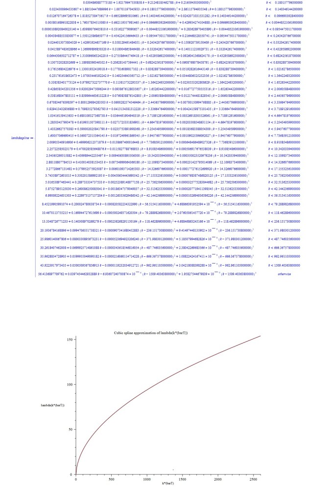
As a first excursion with this new approximation approach, an attempt was made to replicate the results in MW2016 for the cases and , with . Spline function representations of and consisting of 40 cubic pieces were quickly obtained with initial samples of 40 exact values of . These are displayed below as piecewise functions for the case , together with plots of the corresponding splines. The derivatives of were then calculated, and these were used to calculate the entropy functions and the log-saddlepoint-density functions, finally obtaining plots of these which are also shown below for the cases and .
Note that, despite the computational difficulties encountered when trying to compute exact function values for the case in particular, obtaining the corresponding cubic spline function approximations proved to be just as quick and easy as for the case .
Checking accuracy of splines and asymptotic formulae
In the previous section, a solution system was developed based on spline function approximations that can quickly and accurately solve the large deviation problems we are interested in, for any values of , , and , even when these solutions are computationally difficult or impossible to obtain in a fine-grained way using exact functions. This gives us a machine for quickly generating accurate benchmark solutions which, for example, can be compared with analytical work.
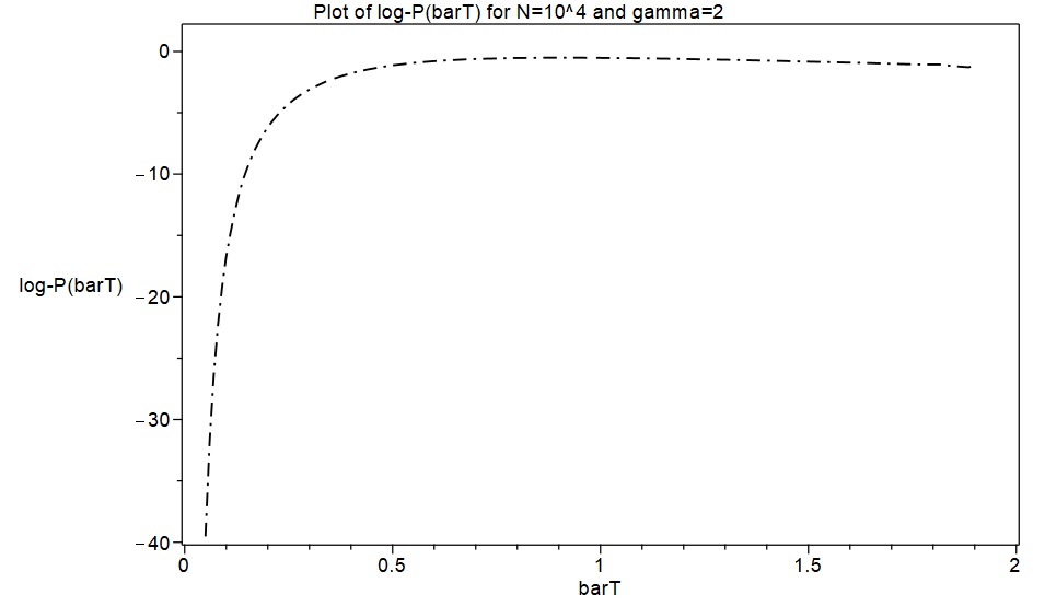
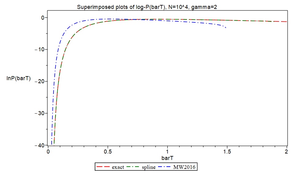
I decided to try to put both the spline function approach and the asymptotic formulae in MW2016 to the test by producing fine-grained exact values for the relevant functions (i.e., approximately 200 function values for values of in the range 0.0 to 2.0), and then comparing our approximations with these. I was able to obtain fine-grained exact values for the case and in MAPLE, and this took a significant amount of computation time using the relevant exact functions. In contrast, it only took a few minutes to produce corresponding spline function approximations to an equally fine-grained degree, i.e. approximately 200 values, with a discretization based on 40 values of , giving a sample of 40 exact values of . I also used formulas [19] and [21] in the Supplement to MW2016 to generate corresponding data based on MW’s asymptotic formulae. I then produced superimposed plots of the exact data, the spline function approximations, and the asymptotic formulae in MW2016 to visually assess accuracy.
As shown in the following plots, the spline function approximations produced results in a few minutes which are essentially indistinguishable from the exact values obtained after numerous hours of computation in MAPLE. However, the asymptotic formulae in MW2016 (plots shown in blue) produced rather inaccurate approximations for and .
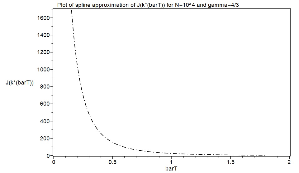
In the case , obtaining fine-grained exact data is computationally very time consuming in MAPLE. Exact formula computations take a lot longer with than with , and producing a fine-grained set of around 200 exact values for all the required functions with and takes a large amount of computing time. However, the spline approximation approach produced such fine-grained results again in only a few minutes. In lieu of fine-grained exact function values, I used MAPLE to generate six exact function values for the case and , and I plotted these as discrete points together with the spline functions to provide some degree of comparison with exact data. The results again indicate that the spline approximations are highly accurate representations of what fine-grained exact results would have looked like.
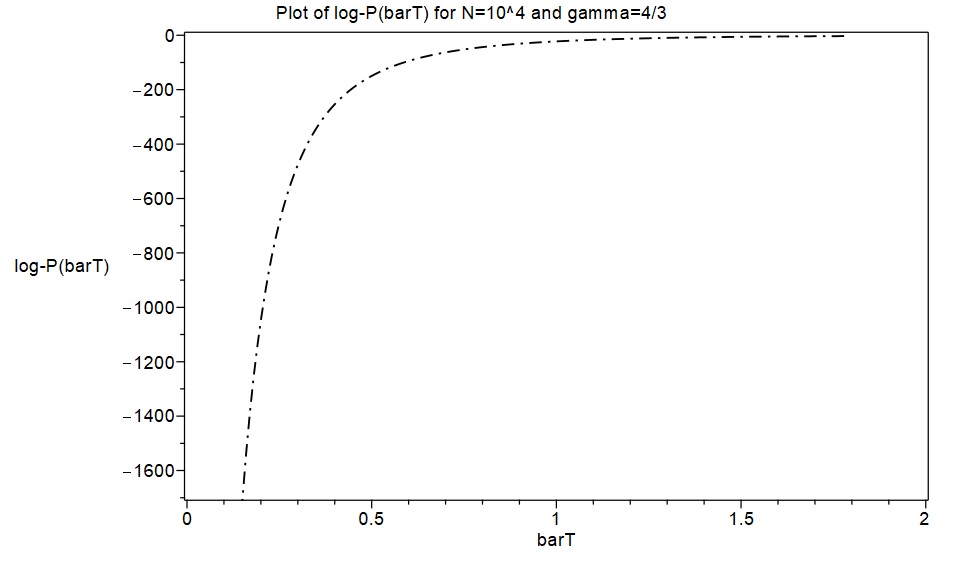
I also decided to compare the asymptotic formulae in MW2016 with the spline approximations and exact function values. I used formulae [19] and [24] in the Supplement to MW2016 for this. (MW asserts there that formula [24] produces more accurate asymptotic approximations than formula [21] in the case ). In the following plots, the spline function approximations are shown in green and MW’s asymptotic formulae in blue. The six exact function values are plotted as discrete red points. As in the case , the spline functions seem to be accurately representing the exact results, while the asymptotic formulae in MW2016 are clearly producing inaccurate results here. The discrepancies between the asymptotic formulae and the spline approximations/exact values seem a lot worse for than for , with .
On the basis of these accuracy checks, there is therefore little question that the asymptotic formulae in MW2016 are producing rather inaccurate results in the case for both and when compared with both exact function values and my spline approximations, notwithstanding the favourable-looking numerical simulation results reported in MW2016 for log-densities. (I have communicated these results to Michael Wilkinson, the author of MW2016).


![S[x] = \int_{t_1}^{t_2} L(x, \dot{x}) dt \qquad \qquad \qquad \qquad \qquad (13)](https://s0.wp.com/latex.php?latex=S%5Bx%5D+%3D+%5Cint_%7Bt_1%7D%5E%7Bt_2%7D+L%28x%2C+%5Cdot%7Bx%7D%29+dt+%5Cqquad+%5Cqquad+%5Cqquad+%5Cqquad+%5Cqquad+%2813%29&bg=ffffff&fg=111111&s=0&c=20201002)


![\int_{t_1}^{t_2} \frac{\partial L}{\partial \dot{x}^{\ast}} \dot{\eta}(t)dt = \bigg[\frac{\partial L}{\partial \dot{x}^{\ast}} \eta(t)\bigg]_{t_1}^{t_2} - \int_{t_1}^{t_2} \frac{d}{dt}\bigg(\frac{\partial L}{\partial \dot{x}^{\ast}}\bigg)\eta(t)dt = - \int_{t_1}^{t_2} \frac{d}{dt}\bigg(\frac{\partial L}{\partial \dot{x}^{\ast}}\bigg)\eta(t)dt](https://s0.wp.com/latex.php?latex=%5Cint_%7Bt_1%7D%5E%7Bt_2%7D+%5Cfrac%7B%5Cpartial+L%7D%7B%5Cpartial+%5Cdot%7Bx%7D%5E%7B%5Cast%7D%7D+%5Cdot%7B%5Ceta%7D%28t%29dt+%3D+%5Cbigg%5B%5Cfrac%7B%5Cpartial+L%7D%7B%5Cpartial+%5Cdot%7Bx%7D%5E%7B%5Cast%7D%7D+%5Ceta%28t%29%5Cbigg%5D_%7Bt_1%7D%5E%7Bt_2%7D+-+%5Cint_%7Bt_1%7D%5E%7Bt_2%7D+%5Cfrac%7Bd%7D%7Bdt%7D%5Cbigg%28%5Cfrac%7B%5Cpartial+L%7D%7B%5Cpartial+%5Cdot%7Bx%7D%5E%7B%5Cast%7D%7D%5Cbigg%29%5Ceta%28t%29dt+%3D+-+%5Cint_%7Bt_1%7D%5E%7Bt_2%7D+%5Cfrac%7Bd%7D%7Bdt%7D%5Cbigg%28%5Cfrac%7B%5Cpartial+L%7D%7B%5Cpartial+%5Cdot%7Bx%7D%5E%7B%5Cast%7D%7D%5Cbigg%29%5Ceta%28t%29dt&bg=ffffff&fg=111111&s=0&c=20201002)


![u(x, t) = \sum_{n=0}^{\infty} b_n \exp\bigg[ -\bigg(\frac{(2n+1)\pi}{2L} \bigg)^2 kt \bigg] \sin\bigg(\frac{(2n+1)\pi}{2L}x\bigg) \qquad \qquad \qquad \qquad \qquad (1)](https://s0.wp.com/latex.php?latex=u%28x%2C+t%29+%3D+%5Csum_%7Bn%3D0%7D%5E%7B%5Cinfty%7D+b_n+%5Cexp%5Cbigg%5B+-%5Cbigg%28%5Cfrac%7B%282n%2B1%29%5Cpi%7D%7B2L%7D+%5Cbigg%29%5E2+kt+%5Cbigg%5D+%5Csin%5Cbigg%28%5Cfrac%7B%282n%2B1%29%5Cpi%7D%7B2L%7Dx%5Cbigg%29+%5Cqquad+%5Cqquad+%5Cqquad+%5Cqquad+%5Cqquad+%281%29&bg=ffffff&fg=111111&s=0&c=20201002)
 required
  , so it was necessary to find the coefficients
  in the following sine series:
 rather than the usual
  . They have period
  and by looking at graphs it is easy to convince oneself that

![= \frac{1}{2} \int_{-2L}^{2L} \bigg[\sin^2\bigg(\frac{(2n+1)\pi}{2L}x\bigg) + \cos^2\bigg(\frac{(2n+1)\pi}{2L}x\bigg) \bigg] dx](https://s0.wp.com/latex.php?latex=%3D+%5Cfrac%7B1%7D%7B2%7D+%5Cint_%7B-2L%7D%5E%7B2L%7D+%5Cbigg%5B%5Csin%5E2%5Cbigg%28%5Cfrac%7B%282n%2B1%29%5Cpi%7D%7B2L%7Dx%5Cbigg%29+%2B+%5Ccos%5E2%5Cbigg%28%5Cfrac%7B%282n%2B1%29%5Cpi%7D%7B2L%7Dx%5Cbigg%29+%5Cbigg%5D+dx&bg=ffffff&fg=111111&s=0&c=20201002)


 . In fact, the functions
  for
for  form a complete, orthogonal set of basis functions and we can expand
  in this basis. To this end, we need to create an odd function involving

![= \frac{u_0}{L} \bigg[-\frac{2L}{(2n+1)\pi}\cos\bigg(\frac{(2n+1)\pi}{2L}x \bigg) \bigg]_0^{2L} = \frac{-2u_0}{(2n+1)\pi} \big(\cos((2n+1)\pi)-1\big)](https://s0.wp.com/latex.php?latex=%3D+%5Cfrac%7Bu_0%7D%7BL%7D+%5Cbigg%5B-%5Cfrac%7B2L%7D%7B%282n%2B1%29%5Cpi%7D%5Ccos%5Cbigg%28%5Cfrac%7B%282n%2B1%29%5Cpi%7D%7B2L%7Dx+%5Cbigg%29+%5Cbigg%5D_0%5E%7B2L%7D+%3D+%5Cfrac%7B-2u_0%7D%7B%282n%2B1%29%5Cpi%7D+%5Cbig%28%5Ccos%28%282n%2B1%29%5Cpi%29-1%5Cbig%29&bg=ffffff&fg=111111&s=0&c=20201002)

![u(x, t) = \frac{4u_0}{\pi}\sum_{n=0}^{\infty} \frac{1}{2n+1} \exp\bigg[ -\bigg(\frac{(2n+1)\pi}{2L} \bigg)^2 kt \bigg] \sin\bigg(\frac{(2n+1)\pi}{2L}x\bigg)](https://s0.wp.com/latex.php?latex=u%28x%2C+t%29+%3D+%5Cfrac%7B4u_0%7D%7B%5Cpi%7D%5Csum_%7Bn%3D0%7D%5E%7B%5Cinfty%7D+%5Cfrac%7B1%7D%7B2n%2B1%7D+%5Cexp%5Cbigg%5B+-%5Cbigg%28%5Cfrac%7B%282n%2B1%29%5Cpi%7D%7B2L%7D+%5Cbigg%29%5E2+kt+%5Cbigg%5D+%5Csin%5Cbigg%28%5Cfrac%7B%282n%2B1%29%5Cpi%7D%7B2L%7Dx%5Cbigg%29&bg=ffffff&fg=111111&s=0&c=20201002)

 which solves (1). The
 is a number to be found by substituting (2) and its relevant derivatives into (1). We assume that
  is not zero, so the first term of the series will be
  . Successive differentiation of (2) and substitution into (1) produces for each power of
  . (The total coefficient of each power of
  is used to find the possible values of
 and we need to find two solutions, one for
  and another for
  . A linear combination of these two solutions can then be used to construct a general solution of (1). The Frobenius procedure also leads to
  = 0 and the following recursion formula for the remaining coefficients:
 first, and can then simply replace
  to get the coefficients for
 results in solutions called Bessel functions of the first kind and order
  . In the present note, I am concerned only with the Bessel function of the first kind and order zero,
  , obtained by setting
  . We then have a starting value
  and we obtain the following coefficients in the power series for


 . I also want to use Watson’s technique of bisecting the range of integration to obtain a clear intuitive understanding of other equivalent integral formulae for
  in the integral in (1) in the extract to get
 into the Taylor series expansion for
  , namely

 to
to  , using a formula I explored in a


 , and divide the integral by
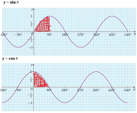

 into the Taylor series expansion for
  , namely


 .
.  . Thus, we obtain the following useful formula for integrating integer powers of sine over a full period:

![= [\sin^{n-1}\theta (-\cos \theta)]_0^{2 \pi} - \int_0^{2 \pi} (n-1)\sin^{n-2} \theta (-\cos^2 \theta)d \theta](https://s0.wp.com/latex.php?latex=%3D+%5B%5Csin%5E%7Bn-1%7D%5Ctheta+%28-%5Ccos+%5Ctheta%29%5D_0%5E%7B2+%5Cpi%7D+-+%5Cint_0%5E%7B2+%5Cpi%7D+%28n-1%29%5Csin%5E%7Bn-2%7D+%5Ctheta+%28-%5Ccos%5E2+%5Ctheta%29d+%5Ctheta&bg=ffffff&fg=111111&s=0&c=20201002)


 is odd and to

 , the distribution of surface charge density per unit area is given by
 ,
,  and
and  , and I wanted to make a note of this here.
 by setting
  in (1) and (2) above to get the sphere


 ,
,  ,
,  . Thus, we can obtain the surface charge density of a circular conducting disk of radius
  -plane and with centre at the origin by setting
  and
and  in (2), and using the fact that on the surface of the ellipsoid we have

 from its centre:
 and did this via a hypergeometric function, which I found quite interesting. I will make a quick note of it here. I came across the following entry in a table of integrals:
![\int \sin^n(ax) dx = -\frac{1}{a} \cos(ax) \ {_2F_1 \big[\frac{1}{2}, \frac{1-n}{2}, \frac{3}{2}, \cos^2(ax)\big]} \qquad \qquad \qquad \qquad \qquad (1)](https://s0.wp.com/latex.php?latex=%5Cint+%5Csin%5En%28ax%29+dx+%3D+-%5Cfrac%7B1%7D%7Ba%7D+%5Ccos%28ax%29+%5C+%7B_2F_1+%5Cbig%5B%5Cfrac%7B1%7D%7B2%7D%2C+%5Cfrac%7B1-n%7D%7B2%7D%2C+%5Cfrac%7B3%7D%7B2%7D%2C+%5Ccos%5E2%28ax%29%5Cbig%5D%7D+%5Cqquad+%5Cqquad+%5Cqquad+%5Cqquad+%5Cqquad+%281%29&bg=ffffff&fg=111111&s=0&c=20201002)
 is a special function known as the
  ,
,  and limits
 ![\int_0^{\pi} dx \sin^5(x) = \bigg[ -\cos(x) \ {_2F_1 \big[\frac{1}{2}, -2, \frac{3}{2}, \cos^2(x)\big]} \bigg]_0^{\pi} = 2 {_2F_1 \big[\frac{1}{2}, -2, \frac{3}{2}, 1 \big]} \qquad \qquad \qquad \qquad \qquad (2)](https://s0.wp.com/latex.php?latex=%5Cint_0%5E%7B%5Cpi%7D+dx+%5Csin%5E5%28x%29+%3D+%5Cbigg%5B+-%5Ccos%28x%29+%5C+%7B_2F_1+%5Cbig%5B%5Cfrac%7B1%7D%7B2%7D%2C+-2%2C+%5Cfrac%7B3%7D%7B2%7D%2C+%5Ccos%5E2%28x%29%5Cbig%5D%7D+%5Cbigg%5D_0%5E%7B%5Cpi%7D+%3D+2+%7B_2F_1+%5Cbig%5B%5Cfrac%7B1%7D%7B2%7D%2C+-2%2C+%5Cfrac%7B3%7D%7B2%7D%2C+1+%5Cbig%5D%7D+%5Cqquad+%5Cqquad+%5Cqquad+%5Cqquad+%5Cqquad+%282%29&bg=ffffff&fg=111111&s=0&c=20201002)
 which yields a simple ratio of products of the
  :
:
![{_2F_1 \big[\frac{1}{2}, -2, \frac{3}{2}, 1 \big]} = \frac{\Gamma \big(\frac{3}{2}\big) \Gamma \big(\frac{3}{2} - \frac{1}{2} + 2 \big)}{\Gamma \big(\frac{3}{2}-\frac{1}{2}\big) \Gamma \big(\frac{3}{2} + 2 \big)} = \frac{\big(\frac{\sqrt{\pi}}{2}\big)(2!)}{(1)\big(\frac{15\sqrt{\pi}}{8}\big)} = \frac{8}{15}](https://s0.wp.com/latex.php?latex=%7B_2F_1+%5Cbig%5B%5Cfrac%7B1%7D%7B2%7D%2C+-2%2C+%5Cfrac%7B3%7D%7B2%7D%2C+1+%5Cbig%5D%7D+%3D+%5Cfrac%7B%5CGamma+%5Cbig%28%5Cfrac%7B3%7D%7B2%7D%5Cbig%29+%5CGamma+%5Cbig%28%5Cfrac%7B3%7D%7B2%7D+-+%5Cfrac%7B1%7D%7B2%7D+%2B+2+%5Cbig%29%7D%7B%5CGamma+%5Cbig%28%5Cfrac%7B3%7D%7B2%7D-%5Cfrac%7B1%7D%7B2%7D%5Cbig%29+%5CGamma+%5Cbig%28%5Cfrac%7B3%7D%7B2%7D+%2B+2+%5Cbig%29%7D+%3D+%5Cfrac%7B%5Cbig%28%5Cfrac%7B%5Csqrt%7B%5Cpi%7D%7D%7B2%7D%5Cbig%29%282%21%29%7D%7B%281%29%5Cbig%28%5Cfrac%7B15%5Csqrt%7B%5Cpi%7D%7D%7B8%7D%5Cbig%29%7D+%3D+%5Cfrac%7B8%7D%7B15%7D&bg=ffffff&fg=111111&s=0&c=20201002)

 can be written
  . If there is an initial condition
  , we can rearrange to get an equation involving two integrals:
 . Note the following integration tricks which are sometimes useful here:

 depends only the ratio
  rather than on
  with initial condition
  . To transform this into a separable equation, make the change of variable
  . Then
  , so we have
  and therefore
  . The initial condition becomes
  , so
, so  . The method of separation of variables can now be applied to the transformed equation.
  , with boundary condition
  that allows us to write the differential equation as


 and therefore the required integrating factor is
  . So what we do is find the integrating factor, then write the equation in the form
  where
where  is a constant of integration. If the integral constant cannot be evaluated directly, it is best to give the solution as

 , the integral
  vanishes and
  so the equation reduces to
  . To solve this, make the change of variable
  . Then
  , so the original equation can be rewritten as
 . It reduces to a linear equation if
  and Bernoulli’s equation if
  . Otherwise, it can be reduced to a linear second-order equation by defining a new dependent variable
  with the equation
  . This converts the original Riccati equation into

 , so equation [15] in MW2016 sets up a relevant Bromwich integral equation, which I will write here as

 variables by induction, we can obtain the following expression for the product term in (2):

 , so the residue at each such singularity is given by
 by creating a semicircle with the straight vertical part located at a point
  to the right of
  , and with the arc of the semicircle large enough to enclose the point
  on the real axis (diagram below). Since
  is the smallest collision rate, and
  is the largest, this ensures that the contour will enclose each
  point.
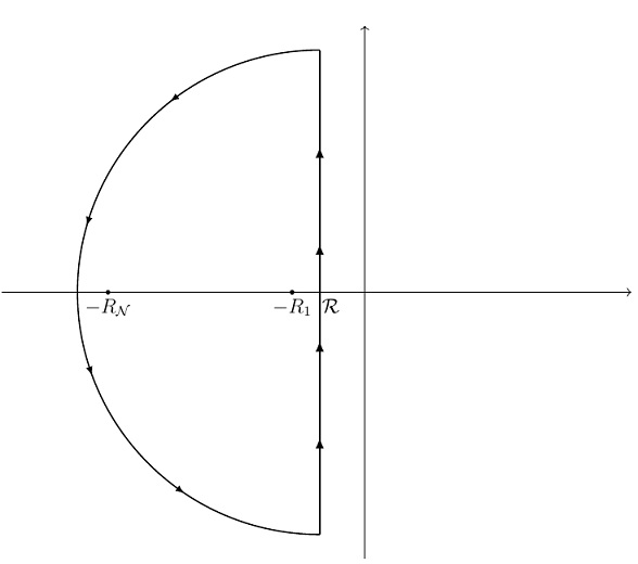


 , we obtain the cumulative distribution function
 , so the expressions in (7) and (8) would involve sums of thousands of product terms, each of these products in turn involving thousands of terms. Therefore, we are still interested in obtaining a formula for the entropy function
  to enable large deviation approximations for (7) and (8) for practical calculations. It may be possible to obtain an approximation for the entropy function directly from the cdf in (8), but this would require further investigation.


 , (17) yields


![= R_{\mathcal{N}+1}\prod_{j=1}^{\mathcal{N}} \bigg(\frac{R_j}{R_j - R_{\mathcal{N}+1}}\bigg) \bigg[\sum_{n=1}^{\mathcal{N}} \prod_{\substack{j=1 \\ j\neq n}}^{\mathcal{N}} \bigg(\frac{1}{R_n - R_j}\bigg) \bigg]](https://s0.wp.com/latex.php?latex=%3D+R_%7B%5Cmathcal%7BN%7D%2B1%7D%5Cprod_%7Bj%3D1%7D%5E%7B%5Cmathcal%7BN%7D%7D+%5Cbigg%28%5Cfrac%7BR_j%7D%7BR_j+-+R_%7B%5Cmathcal%7BN%7D%2B1%7D%7D%5Cbigg%29+%5Cbigg%5B%5Csum_%7Bn%3D1%7D%5E%7B%5Cmathcal%7BN%7D%7D+%5Cprod_%7B%5Csubstack%7Bj%3D1+%5C%5C+j%5Cneq+n%7D%7D%5E%7B%5Cmathcal%7BN%7D%7D+%5Cbigg%28%5Cfrac%7B1%7D%7BR_n+-+R_j%7D%5Cbigg%29+%5Cbigg%5D&bg=ffffff&fg=111111&s=0&c=20201002)
![+ \prod_{j=1}^{\mathcal{N}} \bigg(\frac{R_j}{R_j - R_{\mathcal{N}+1}}\bigg) \bigg[\sum_{n=1}^{\mathcal{N}} \prod_{\substack{j=1 \\ j\neq n}}^{\mathcal{N}} \bigg(\frac{R_j}{R_j - R_n}\bigg) \bigg]](https://s0.wp.com/latex.php?latex=%2B+%5Cprod_%7Bj%3D1%7D%5E%7B%5Cmathcal%7BN%7D%7D+%5Cbigg%28%5Cfrac%7BR_j%7D%7BR_j+-+R_%7B%5Cmathcal%7BN%7D%2B1%7D%7D%5Cbigg%29+%5Cbigg%5B%5Csum_%7Bn%3D1%7D%5E%7B%5Cmathcal%7BN%7D%7D+%5Cprod_%7B%5Csubstack%7Bj%3D1+%5C%5C+j%5Cneq+n%7D%7D%5E%7B%5Cmathcal%7BN%7D%7D+%5Cbigg%28%5Cfrac%7BR_j%7D%7BR_j+-+R_n%7D%5Cbigg%29+%5Cbigg%5D&bg=ffffff&fg=111111&s=0&c=20201002)

 which is easy to prove by repeated bivariate partial fraction expansions, and clearly exhibits the pattern represented by (3):


![+ \bigg[\sum_{n=1}^{\mathcal{N}} \prod_{\substack{j=1 \\ j\neq n}}^{\mathcal{N}} \bigg(\frac{R_j}{R_j - R_n}\bigg)\bigg(\frac{R_n}{R_n - R_{\mathcal{N}+1}}\bigg)R_{\mathcal{N}+1}\bigg]\bigg(\frac{1}{R_{\mathcal{N}+1}+z}\bigg)](https://s0.wp.com/latex.php?latex=%2B+%5Cbigg%5B%5Csum_%7Bn%3D1%7D%5E%7B%5Cmathcal%7BN%7D%7D+%5Cprod_%7B%5Csubstack%7Bj%3D1+%5C%5C+j%5Cneq+n%7D%7D%5E%7B%5Cmathcal%7BN%7D%7D+%5Cbigg%28%5Cfrac%7BR_j%7D%7BR_j+-+R_n%7D%5Cbigg%29%5Cbigg%28%5Cfrac%7BR_n%7D%7BR_n+-+R_%7B%5Cmathcal%7BN%7D%2B1%7D%7D%5Cbigg%29R_%7B%5Cmathcal%7BN%7D%2B1%7D%5Cbigg%5D%5Cbigg%28%5Cfrac%7B1%7D%7BR_%7B%5Cmathcal%7BN%7D%2B1%7D%2Bz%7D%5Cbigg%29&bg=ffffff&fg=111111&s=0&c=20201002)

![+ \bigg[\prod_{j=1}^{\mathcal{N}} \bigg(\frac{R_j}{R_j - R_{\mathcal{N}+1}}\bigg)R_{\mathcal{N}+1}\bigg]\bigg(\frac{1}{R_{\mathcal{N}+1}+z}\bigg)](https://s0.wp.com/latex.php?latex=%2B+%5Cbigg%5B%5Cprod_%7Bj%3D1%7D%5E%7B%5Cmathcal%7BN%7D%7D+%5Cbigg%28%5Cfrac%7BR_j%7D%7BR_j+-+R_%7B%5Cmathcal%7BN%7D%2B1%7D%7D%5Cbigg%29R_%7B%5Cmathcal%7BN%7D%2B1%7D%5Cbigg%5D%5Cbigg%28%5Cfrac%7B1%7D%7BR_%7B%5Cmathcal%7BN%7D%2B1%7D%2Bz%7D%5Cbigg%29&bg=ffffff&fg=111111&s=0&c=20201002)

 , so (3) is proved.
 took hours and it was even more time consuming to obtain the necessary fine-grained exact function values for the case
  . In view of these difficulties, it seemed desirable to attempt to develop a new numerical solution system for large deviation problems that would enable accurate numerical results to be produced in MAPLE, using only the simplest mathematical functions. This note reports my experiments with one way of achieving this using cubic spline functions.
 and
and  . Also assume a given collision rate parameter
 ![\gamma \in [4/3,2]](https://s0.wp.com/latex.php?latex=%5Cgamma+%5Cin+%5B4%2F3%2C2%5D&bg=ffffff&fg=111111&s=0&c=20201002) , and that
, and that  . The cumulant generating function in equation [14] in MW2016 is then a smooth, strictly concave function in both
  . To see this, write it as


 ,
,  are the even-indexed Bernoulli numbers, and
  is a remainder term. Numerical experiments with MAPLE indicate that only the first two terms on the right-hand side of the Euler-Maclaurin formula are needed to obtain accurate approximations of our cumulant generating function over the entire range of relevant values of
  . Thus, to a close approximation we have


 for
for  ,
,  , and
, and 
 and
and 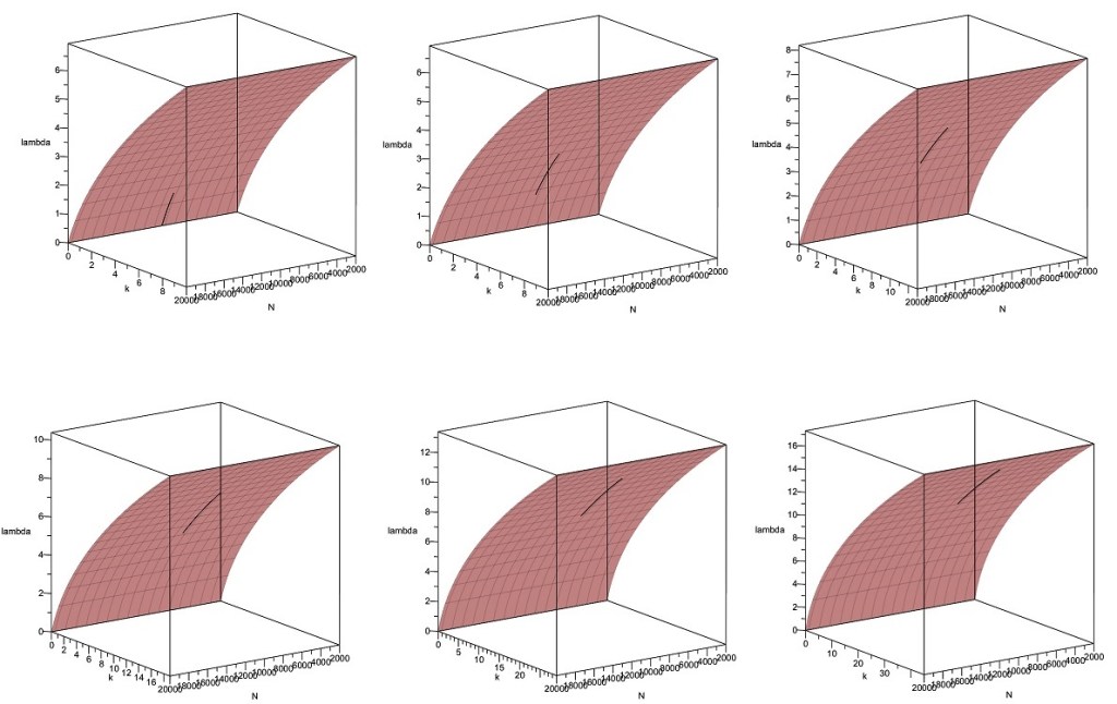
 to
to  , as shown below:
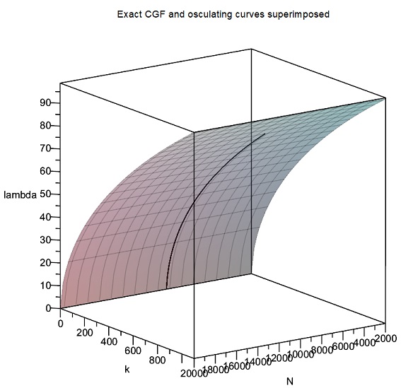
 on the corresponding


 , using (11) above, we obtain
 . There is no correction needed if
  , and this happens when
  in (15) above. But this is exactly the saddlepoint condition in equation [16] in MW2016, so one of the key equations in the large deviation theory in MW2016 has now appeared naturally in this simple quadratic setup.
 in order to find exact values of
  with large values of


 , analogous to the quadratic spline created manually for the cumulant generating function in the previous section. This quadratic spline worked very well due to the smoothness and well-behaved nature of the cumulant generating function, but even more accurate results can be obtained with cubic splines. MAPLE routines can be written which can generate such cubic spline approximations very quickly.
 and the log-saddlepoint-density function
  . (The term fine-grained is used here to mean approximately 200 values of the relevant functions, or more, corresponding to values of
  and
and